
Statistics · Distributions
Sampling Distributions and Standard Errors
Why every survey estimate would change if the sample were drawn again, how the standard error measures that change, and how to calculate, report and interpret it correctly in business research.
Every figure in a survey report is an estimate. If 36% of 400 customers say they are very satisfied, the true share among all customers is unlikely to be exactly 36%, and a second sample of 400 drawn in the same way would almost certainly give a slightly different number. The sampling distribution describes how an estimate would vary across all the samples that could have been drawn. The standard error is the standard deviation of that distribution: a single number that summarises how far an estimate typically falls from the value it is trying to measure. Together they are the foundation of confidence intervals, margins of error and significance tests, and they are among the most frequently misunderstood ideas in applied statistics (Altman & Bland, 2005).
From one sample to many
Imagine a population of customers whose monthly spend has a mean of $82 and a standard deviation of $58. Draw a random sample of 25 customers and calculate their mean spend. Now repeat the exercise thousands of times, each time recording the sample mean. The collection of all those sample means is the sampling distribution of the mean.
Three facts about this distribution matter in practice. First, its centre is the population mean: the sample mean is an unbiased estimator, so on average it neither overstates nor understates the truth. Second, its spread is much smaller than the spread of individual spending, because averaging cancels out much of the individual variation. Third, as the sample size grows, its shape becomes increasingly close to a normal distribution, even when the population itself is strongly skewed. This third fact is the central limit theorem, and it is the reason normal-based intervals work for so many business measures (Wasserman, 2004).
The sampling distribution is a thought experiment. In practice we draw only one sample. The power of statistical theory is that it lets us describe the variability of the estimate from the information in that single sample.
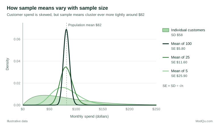
The standard error
For the mean of a simple random sample of size n from a population with standard deviation σ, the standard error is:
SE(x̄) = σ ÷ √n
Because σ is rarely known, it is replaced by the sample standard deviation s. Student (1908) showed that this substitution calls for the t distribution rather than the normal distribution when samples are small, a correction that matters little once the sample exceeds a few dozen.
For a percentage, the corresponding formula is:
SE(p) = √(p × (1 − p) ÷ n)
This is the formula behind the margins of error quoted for opinion polls. It reaches its maximum when p is 50%, so pollsters often quote the margin for 50% as a conservative figure for the whole survey.
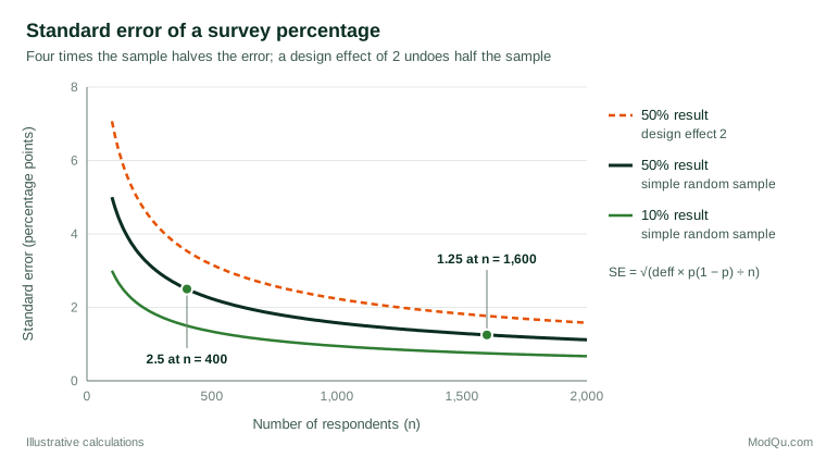
The square root of n in the denominator has a sobering implication. To halve the standard error, the sample must be four times as large. Wainer (2007) called this relationship, first described by Abraham de Moivre, "the most dangerous equation" because ignoring it leads people to misread the extremes produced by small groups. The smallest schools, hospitals, sales territories or stores tend to show both the best and the worst results simply because their averages are based on fewer observations and vary more. The same misplaced trust in small samples is what Tversky and Kahneman (1971) described as the belief in the "law of small numbers".
Standard deviation is not standard error
The standard deviation describes how much individual observations differ from one another. The standard error describes how precisely a statistic, such as a mean or a percentage, has been estimated. As the sample grows, the standard deviation settles near its population value, while the standard error keeps shrinking towards zero. Confusing the two is a common reporting error: the standard deviation is the right measure for describing variation among customers, and the standard error is the right measure for describing uncertainty in an estimate (Altman & Bland, 2005).
A worked example
Suppose, hypothetically, that a retailer surveys a simple random sample of 400 customers. Mean monthly spend is $82 with a standard deviation of $58, and 36% say they are very satisfied.
- Mean spend. The standard error is 58 ÷ √400 = $2.90. A 95% confidence interval is about 82 ± 1.97 × 2.90, or roughly $76.30 to $87.70.
- Satisfaction. The standard error is √(0.36 × 0.64 ÷ 400) = 0.024, or 2.4 percentage points. The 95% margin of error is about ±4.7 points, giving an interval from 31.3% to 40.7%.
- A change between waves. In the next wave, a fresh sample of 400 gives 43% very satisfied, with an interval from 38.1% to 47.9%. The two intervals overlap, yet the change is statistically significant. The standard error of the difference between independent estimates is √(SE1² + SE2²) = √(2.4² + 2.5²) ≈ 3.4 points, so the 95% interval for the seven-point rise runs from about 0.2 to 13.8 points, which excludes zero.
The last point illustrates a well-documented trap. Checking whether two confidence intervals overlap is a conservative and often misleading test of whether two estimates differ (Schenker & Gentleman, 2001). Comparisons should be based on the standard error of the difference itself.
Subgroups need the same care. If 100 of the 400 customers are under 30 and 36% of them are very satisfied, the standard error for that subgroup is √(0.36 × 0.64 ÷ 100) = 4.8 points, twice the figure for the full sample, and the margin of error is about ±9.4 points. A subgroup result that looks strikingly different from the total may simply reflect this extra noise.
Standard errors in real survey designs
The formulas above assume simple random sampling from a very large population. Real business surveys rarely meet that ideal, and the departures change the standard error, sometimes substantially (Lohr, 2021).
Finite populations
When the sample is a sizeable fraction of the population, such as 400 of a firm's 2,000 business clients, there is less left to be uncertain about. The standard error is multiplied by the finite population correction, √(1 − n ÷ N), here √(1 − 0.2) ≈ 0.89 (Cochran, 1977). The correction can usually be ignored when the sample is less than about 5% of the population.
Stratification, clustering and weighting
Stratified sampling usually reduces the standard error, because it removes variation between strata from the estimate; Neyman (1934) showed how to allocate a sample across strata to minimise it. Cluster sampling usually increases the standard error, because people in the same store, branch or neighbourhood tend to resemble one another and so provide overlapping information. Kish (1965) summarised these effects with the design effect, the ratio of the actual variance of an estimate to the variance under a simple random sample of the same size. For a cluster sample with m respondents per cluster and intraclass correlation ρ, the design effect is approximately:
deff = 1 + (m − 1) × ρ
Interviewing 20 customers in each of 20 stores, with an intraclass correlation of only 0.05, gives a design effect of about 1.95: the 400 interviews carry roughly the information of 205 independent ones. Unequal weights inflate the variance in a similar way.
In the worked example, a design effect of 1.6 would raise the standard error of the satisfaction figure from 2.4 to about 3.0 points and widen the margin of error from ±4.7 to about ±5.9. The effective sample size would be 400 ÷ 1.6 = 250. Analysis software that treats weighted, clustered data as a simple random sample reports standard errors that are too small, which in turn makes differences look more significant than they are (Lumley, 2010). Design-based variance estimation methods, such as Taylor linearisation and replication, are described in detail by Wolter (2007).
Dependence in business data
Clustering is not confined to formal survey designs. Transactions from the same customer, visits on the same day or employees in the same team are correlated in the same way. Moulton (1990) showed that ignoring such grouping when relating individual outcomes to group-level variables can make standard errors far too small. Unequal variability across observations raises a related problem in regression, for which heteroskedasticity-consistent "robust" standard errors are a standard remedy (White, 1980).
When there is no simple formula
Formulas exist for means, percentages and many regression coefficients, but not for every statistic a business analyst needs. The median basket value, the ratio of two totals, a Net Promoter Score or the gap between two segments' medians may have no convenient standard error formula. The bootstrap, introduced by Efron (1979), estimates the sampling distribution by resampling the observed data with replacement many times and recalculating the statistic each time. The standard deviation of the resampled statistics estimates the standard error (Efron & Tibshirani, 1994). Hesterberg (2015) gives an accessible account of when the bootstrap works well and when it does not, noting in particular that it does not rescue very small samples. For complex survey samples, the resampling must respect the design, which is why replication methods such as the jackknife and balanced repeated replication are used (Wolter, 2007).
What the standard error does not measure
The standard error measures only sampling error, the variation that arises because a sample rather than the whole population was observed. It says nothing about coverage error, nonresponse bias, poorly worded questions or processing mistakes, which together make up the total survey error (Groves & Lyberg, 2010). A large but biased sample can have a tiny standard error and still be badly wrong. Meng (2018) showed that, for a non-random sample, even a very weak correlation between who responds and what they report can outweigh an enormous sample size, so that millions of self-selected responses may be worth no more than a few hundred random ones. A small standard error is evidence of precision, not of accuracy.
The interpretation of the resulting intervals also needs care. In the frequentist framework set out by Neyman (1937), a 95% confidence interval comes from a procedure that captures the true value in 95% of repeated samples; any one interval either contains it or does not. Fisher (1922) had earlier framed estimation in terms of the sampling distributions of statistics, which remains the logic behind standard errors today.
Reporting standard errors well
Error bars are a common way to show uncertainty, but they are easily misread. In a survey of researchers in psychology, behavioural neuroscience and medicine, Belia et al. (2005) found widespread misunderstanding of how standard error bars and confidence interval bars relate to statistical significance. Cumming and Finch (2005) give practical rules for reading such charts. Good practice includes:
- State what the bars show. Label error bars as standard errors or as 95% confidence intervals. A 95% interval is roughly twice as wide as a standard error bar.
- Use the design-based standard error. Report standard errors and margins of error that reflect weighting and clustering, and state the design effect or effective sample size where it is substantial.
- Show the base. Give the unweighted number of respondents behind every percentage, especially for subgroups.
- Compare differences directly. Test or show the interval for the difference rather than relying on overlapping bars.
- Avoid false precision. A percentage with a standard error of three points should not be reported to one decimal place.
Common mistakes
- Reporting the standard deviation as if it were the standard error, or the reverse. The first exaggerates uncertainty; the second understates the variation among people.
- Applying simple random sample formulas to complex samples. This understates uncertainty whenever the design effect exceeds 1.
- Using the overall margin of error for subgroups. A subgroup of 100 has a standard error twice that of the full sample of 400.
- Treating a small standard error as proof of accuracy. Bias does not shrink with sample size.
- Ranking small units on raw averages. Small stores, teams or regions appear at both extremes because their estimates are noisier.
Key takeaways
A sampling distribution describes how an estimate would vary from sample to sample, and the standard error summarises that variation in one number. Standard errors shrink with the square root of the sample size, so precision becomes expensive quickly. They grow with clustering and unequal weighting and shrink with good stratification, so the sampling design must be reflected in the calculation. When no formula exists, the bootstrap offers a practical alternative. Above all, the standard error measures only random sampling error. It is an essential guide to precision, but it must be read alongside an honest assessment of bias.
References
Altman, D. G., & Bland, J. M. (2005). Standard deviations and standard errors. BMJ, 331(7521), 903. https://doi.org/10.1136/bmj.331.7521.903
Belia, S., Fidler, F., Williams, J., & Cumming, G. (2005). Researchers misunderstand confidence intervals and standard error bars. Psychological Methods, 10(4), 389–396. https://doi.org/10.1037/1082-989X.10.4.389
Cochran, W. G. (1977). Sampling techniques (3rd ed.). Wiley.
Cumming, G., & Finch, S. (2005). Inference by eye: Confidence intervals and how to read pictures of data. American Psychologist, 60(2), 170–180. https://doi.org/10.1037/0003-066X.60.2.170
Efron, B. (1979). Bootstrap methods: Another look at the jackknife. The Annals of Statistics, 7(1), 1–26. https://doi.org/10.1214/aos/1176344552
Efron, B., & Tibshirani, R. J. (1994). An introduction to the bootstrap. Chapman and Hall/CRC. https://doi.org/10.1201/9780429246593
Fisher, R. A. (1922). On the mathematical foundations of theoretical statistics. Philosophical Transactions of the Royal Society of London. Series A, Containing Papers of a Mathematical or Physical Character, 222(594–604), 309–368. https://doi.org/10.1098/rsta.1922.0009
Groves, R. M., & Lyberg, L. (2010). Total survey error: Past, present, and future. Public Opinion Quarterly, 74(5), 849–879. https://doi.org/10.1093/poq/nfq065
Hesterberg, T. C. (2015). What teachers should know about the bootstrap: Resampling in the undergraduate statistics curriculum. The American Statistician, 69(4), 371–386. https://doi.org/10.1080/00031305.2015.1089789
Kish, L. (1965). Survey sampling. Wiley.
Lohr, S. L. (2021). Sampling: Design and analysis (3rd ed.). Chapman and Hall/CRC. https://doi.org/10.1201/9780429298899
Lumley, T. (2010). Complex surveys: A guide to analysis using R. Wiley. https://doi.org/10.1002/9780470580066
Meng, X.-L. (2018). Statistical paradises and paradoxes in big data (I): Law of large populations, big data paradox, and the 2016 US presidential election. The Annals of Applied Statistics, 12(2), 685–726. https://doi.org/10.1214/18-AOAS1161SF
Moulton, B. R. (1990). An illustration of a pitfall in estimating the effects of aggregate variables on micro units. The Review of Economics and Statistics, 72(2), 334–338. https://doi.org/10.2307/2109724
Neyman, J. (1934). On the two different aspects of the representative method: The method of stratified sampling and the method of purposive selection. Journal of the Royal Statistical Society, 97(4), 558–625. https://doi.org/10.2307/2342192
Neyman, J. (1937). Outline of a theory of statistical estimation based on the classical theory of probability. Philosophical Transactions of the Royal Society of London. Series A, Mathematical and Physical Sciences, 236(767), 333–380. https://doi.org/10.1098/rsta.1937.0005
Schenker, N., & Gentleman, J. F. (2001). On judging the significance of differences by examining the overlap between confidence intervals. The American Statistician, 55(3), 182–186. https://doi.org/10.1198/000313001317097960
Student. (1908). The probable error of a mean. Biometrika, 6(1), 1–25. https://doi.org/10.1093/biomet/6.1.1
Tversky, A., & Kahneman, D. (1971). Belief in the law of small numbers. Psychological Bulletin, 76(2), 105–110. https://doi.org/10.1037/h0031322
Wainer, H. (2007). The most dangerous equation. American Scientist, 95(3), 249. https://doi.org/10.1511/2007.65.1026
Wasserman, L. (2004). All of statistics: A concise course in statistical inference. Springer. https://doi.org/10.1007/978-0-387-21736-9
White, H. (1980). A heteroskedasticity-consistent covariance matrix estimator and a direct test for heteroskedasticity. Econometrica, 48(4), 817–838. https://doi.org/10.2307/1912934
Wolter, K. M. (2007). Introduction to variance estimation (2nd ed.). Springer. https://doi.org/10.1007/978-0-387-35099-8