
Statistics · Distributions
Long-Tailed and Power-Law Distributions
Why customer spend, product sales and many other business quantities have long tails, what power laws are, how to test for them properly, and how to summarise data dominated by a few extreme values.
In many business data sets, a small number of observations account for a large share of the total. A handful of customers generate most of the revenue, a few products dominate sales, a few claims make up most of the losses, and a few viral posts collect most of the attention. Data like these do not cluster politely around an average. They have a long tail: a stretch of rare but very large values that extends far beyond the typical case. The most famous family of long-tailed distributions is the power law, which has been reported for word frequencies, city sizes, firm sizes, incomes, citations and links on the web (Newman, 2005).
Long tails matter because the usual statistical toolkit, built around the mean, the standard deviation and the normal curve, can mislead badly when a few extreme values dominate. This article explains what long-tailed and power-law distributions are, where they come from, how to test whether data really follow a power law, and how to report such data in survey and business research.
What makes a tail long?
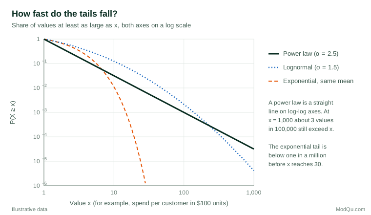
The tail of a distribution describes how quickly the probability of very large values falls away. In a normal distribution it falls extremely fast: values more than four standard deviations above the mean occur about three times in 100,000 observations, and values ten standard deviations out practically never occur.
A distribution is called heavy-tailed when its tail falls more slowly than any exponential. The terms long-tailed, fat-tailed and heavy-tailed are often used interchangeably in applied work, although technical definitions differ slightly between fields. What they share is the practical consequence: extreme values are far more common than a normal or exponential model would predict, and they carry a large share of the total.
Two heavy-tailed families appear again and again in practice:
- Power-law (Pareto) distributions, in which the probability of a value decreases as a power of the value itself.
- Lognormal distributions, in which the logarithm of the value is normally distributed. The lognormal arises naturally when many small effects multiply together, and it describes quantities such as incomes, incubation periods and particle sizes across many sciences (Limpert et al., 2001).
The power law and the Pareto distribution
A quantity x follows a power law if its probability density is proportional to a negative power of x, above some minimum value xmin:
p(x) = C x−α, for x ≥ xmin
Here α is the scaling exponent and C is a constant that makes the probabilities add up to one. In the notation of Clauset et al. (2009), the share of values at least as large as x is then:
P(X ≥ x) = (x ÷ xmin)−(α − 1)
This is the Pareto distribution, named after the economist Vilfredo Pareto, who studied the distribution of incomes; Arnold (2015) gives a book-length treatment of the family and its variants. A related form, Zipf's law, describes the same pattern by rank: the second most common word in a language appears about half as often as the most common, the third about a third as often, and so on (Newman, 2005).
The defining property of a power law is scale invariance. Taking logarithms of both sides gives a straight line: log P(X ≥ x) falls linearly with log x. Doubling x always reduces the probability by the same factor, whether we move from $1,000 to $2,000 or from $100,000 to $200,000. There is no "typical" scale beyond which large values become negligible.
Where long tails appear
Price (1965) showed that a small number of scientific papers receive a very large share of citations, a pattern repeated in many later studies. Barabási and Albert (1999) reported that the number of links per page on the web follows a power law and proposed a model of growing networks to explain it. Axtell (2001) found that the sizes of US firms follow a Zipf distribution closely, and Gabaix (1999) offered an explanation for the long-observed Zipf's law for city sizes.
Finance supplied one of the earliest and most influential examples. Mandelbrot (1963) showed that changes in cotton prices had far heavier tails than a normal distribution allows, so that large price moves were much more frequent than standard models predicted. Large daily moves in asset returns are now recognised as one of the "stylised facts" of financial markets (Cont, 2001). Gabaix (2009) reviews power laws in economics and finance more broadly, including incomes, wealth, firm sizes and trading volumes.
In consumer markets, the long tail became a popular business idea in the mid-2000s: online retailers, it was argued, can profit from selling small quantities of a very large number of niche products. Brynjolfsson et al. (2003) estimated that a substantial share of online book sales came from obscure titles that a typical large physical bookshop would not stock, and that this extra variety created considerable value for consumers. Brynjolfsson et al. (2011) later found that, for the same retailer, sales through the online channel were less concentrated than catalogue sales, and linked the difference to lower search costs. Survey data show the same shape in spend per customer, household wealth and time spent on apps.
Why long tails arise
Several mechanisms can generate power laws and other heavy tails, and different mechanisms imply different things for prediction and policy (Mitzenmacher, 2004).
- Cumulative advantage. Simon (1955) showed that if new units are more likely to join groups that are already large, a power law emerges. This "rich get richer" process underlies the network model of Barabási and Albert (1999) and the citation patterns described by Price (1965).
- Proportional random growth. When each unit grows by a random percentage each period, sizes tend towards a lognormal distribution; with small modifications, such as a lower barrier on size, the result becomes a power law (Gabaix, 1999, 2009).
- Social influence. In an online experiment with artificial music markets, Salganik et al. (2006) found that letting people see what others had downloaded made success both more unequal and less predictable.
Because cumulative advantage and multiplicative growth can produce power laws and lognormals that look very similar in finite samples, a good fit to one family does not, on its own, identify the mechanism (Mitzenmacher, 2004).
Why long tails break familiar statistics
The mean of a power law is finite only when α > 2, and the variance is finite only when α > 3 (Newman, 2005). Many real data sets have exponents between 2 and 3, which means the population mean exists but the population variance, in theory, does not. In practice this has several uncomfortable consequences:
- Sample means are unstable. A single new observation can shift the average dramatically. The mean converges very slowly as the sample grows, and the central limit theorem gives a poor approximation at ordinary sample sizes.
- Standard deviations mislead. A sample standard deviation can always be computed, but it does not estimate a stable population quantity when the variance is infinite, so confidence intervals built from it can be far too narrow.
- Rare events dominate risk. In heavy-tailed settings a single extreme loss or windfall can outweigh years of ordinary outcomes, so planning around the average case ignores the cases that matter most.
A worked example: customer revenue concentration
Suppose, hypothetically, that annual spend per customer follows a Pareto distribution with α = 2.16 and a minimum spend of $100. These values imply a mean spend of $725 but a median of only $182. A few very large accounts pull the mean upward.
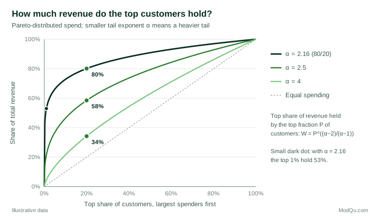
Concentration follows directly from the exponent. Under a power law with α > 2, the share of the total held by the top fraction P of units is:
W = P(α − 2) ÷ (α − 1)
With α = 2.16, the top 20% of customers hold 80% of revenue, which is the familiar 80/20 rule, and the top 1% alone hold 53% (Newman, 2005, derives the same relationship). With α = 2.5, the top 20% hold 58%, and with α = 4 they hold 34%. Small changes in the exponent therefore mean large changes in concentration.
Now imagine a customer survey of 400 respondents drawn from this population. Because the variance is infinite, two such samples can give very different average spends, depending on whether one of the rare very large customers happens to be included. A report that says "average spend rose 15% since last year" may be describing nothing more than a single respondent. The median, quantiles and top shares are far more stable summaries.
Testing for a power law properly
Many published claims of power laws rest on weak evidence (Stumpf & Porter, 2012). The most common approach, plotting a histogram on log-log axes and fitting a straight line by least squares, produces biased estimates of α and cannot by itself show that a power law is the right model (Goldstein et al., 2004; Clauset et al., 2009). Clauset et al. (2009) recommend a more careful procedure:
- Estimate α by maximum likelihood. For continuous data above xmin, the estimate is α̂ = 1 + n [Σ ln(xi ÷ xmin)]−1, where n is the number of observations in the tail. The closely related Hill estimator of the tail index is still widely used (Resnick, 2007).
- Choose xmin from the data. Power-law behaviour usually holds only in the upper tail. Clauset et al. (2009) choose the threshold that makes the fitted model closest to the data, measured by the Kolmogorov–Smirnov statistic.
- Test goodness of fit. Compare the observed fit with fits to synthetic data sets drawn from the fitted model to see whether the power law is plausible at all.
- Compare with alternatives. Use likelihood-ratio tests against the lognormal, the exponential and the power law with an exponential cut-off. Often the data cannot distinguish between them.
When Clauset et al. (2009) applied this procedure to 24 real-world data sets, several well-known "power laws" were only weakly supported or were fitted equally well by a lognormal. Broido and Clauset (2019) analysed nearly 1,000 networks and concluded that strongly scale-free networks are rare. Stumpf and Porter (2012) suggest that a power law should be supported across at least two orders of magnitude of data and, ideally, by a plausible mechanism.
For practical risk analysis, extreme value theory provides a complementary toolkit. Rather than modelling the whole distribution, it models only the values above a high threshold, typically with a generalised Pareto distribution, and uses that model to estimate the size and frequency of rare events (Coles, 2001).
Practical guidance for survey and business data
- Report medians and quantiles alongside means. For spend, income or usage data, show the median and upper percentiles such as the 90th and 99th. If the mean is reported, say how much of the total comes from the top 1% or 5%.
- Report concentration directly. Top shares (the share held by the top 10% or 20%), Lorenz curves and Gini coefficients describe long-tailed data better than a mean and standard deviation.
- Work on the log scale. Log-transforming positive, skewed values often makes them close to normal and makes models more stable, although results must then be interpreted as percentage or ratio effects.
- Plan samples around the tail. If a few large customers drive the total, a simple random sample will include too few of them. Stratify by size and oversample the largest units, then apply weights, as business surveys commonly do.
- Handle extreme values deliberately. Trimming, winsorising or top-coding can stabilise estimates, but each removes real information. Document the rule and show results with and without it.
- Segment the head and the tail. Large accounts often behave differently from the bulk of the market.
Common mistakes
- Treating the mean as typical. In long-tailed data most units are below the mean, often far below it.
- Calling every skewed distribution a power law. Straight-looking log-log plots are easy to produce. Without formal tests and a comparison with the lognormal, the label is not justified.
- Fitting lines to log-log histograms. This gives biased exponents and misleading confidence (Goldstein et al., 2004).
- Extrapolating far beyond the data. Even a well-fitted tail model becomes uncertain at the extremes.
- Ignoring the role of feedback. Where success depends on visibility or popularity, past rankings may be poor guides to future ones (Salganik et al., 2006).
Key takeaways
Long-tailed distributions are the rule rather than the exception for many business quantities: spend, sales, firm size, wealth and online attention. In these data, a few large values carry much of the total, means and standard deviations become unstable, and the familiar normal-curve intuitions fail. Power laws are one important model for such tails, but they should be claimed only after maximum-likelihood fitting, goodness-of-fit testing and comparison with alternatives such as the lognormal. For reporting, medians, quantiles and concentration measures tell decision-makers far more than an average alone.
References
Arnold, B. C. (2015). Pareto distributions. Chapman and Hall/CRC. https://doi.org/10.1201/b18141
Axtell, R. L. (2001). Zipf distribution of U.S. firm sizes. Science, 293(5536), 1818–1820. https://doi.org/10.1126/science.1062081
Barabási, A.-L., & Albert, R. (1999). Emergence of scaling in random networks. Science, 286(5439), 509–512. https://doi.org/10.1126/science.286.5439.509
Broido, A. D., & Clauset, A. (2019). Scale-free networks are rare. Nature Communications, 10, Article 1017. https://doi.org/10.1038/s41467-019-08746-5
Brynjolfsson, E., Hu, Y., & Smith, M. D. (2003). Consumer surplus in the digital economy: Estimating the value of increased product variety at online booksellers. Management Science, 49(11), 1580–1596. https://doi.org/10.1287/mnsc.49.11.1580.20580
Brynjolfsson, E., Hu, Y., & Simester, D. (2011). Goodbye Pareto principle, hello long tail: The effect of search costs on the concentration of product sales. Management Science, 57(8), 1373–1386. https://doi.org/10.1287/mnsc.1110.1371
Clauset, A., Shalizi, C. R., & Newman, M. E. J. (2009). Power-law distributions in empirical data. SIAM Review, 51(4), 661–703. https://doi.org/10.1137/070710111
Coles, S. (2001). An introduction to statistical modeling of extreme values. Springer. https://doi.org/10.1007/978-1-4471-3675-0
Cont, R. (2001). Empirical properties of asset returns: Stylized facts and statistical issues. Quantitative Finance, 1(2), 223–236. https://doi.org/10.1080/713665670
Gabaix, X. (1999). Zipf's law for cities: An explanation. The Quarterly Journal of Economics, 114(3), 739–767. https://doi.org/10.1162/003355399556133
Gabaix, X. (2009). Power laws in economics and finance. Annual Review of Economics, 1(1), 255–294. https://doi.org/10.1146/annurev.economics.050708.142940
Goldstein, M. L., Morris, S. A., & Yen, G. G. (2004). Problems with fitting to the power-law distribution. The European Physical Journal B, 41(2), 255–258. https://doi.org/10.1140/epjb/e2004-00316-5
Limpert, E., Stahel, W. A., & Abbt, M. (2001). Log-normal distributions across the sciences: Keys and clues. BioScience, 51(5), 341–352. https://doi.org/10.1641/0006-3568(2001)051[0341:LNDATS]2.0.CO;2
Mandelbrot, B. (1963). The variation of certain speculative prices. The Journal of Business, 36(4), 394–419. https://doi.org/10.1086/294632
Mitzenmacher, M. (2004). A brief history of generative models for power law and lognormal distributions. Internet Mathematics, 1(2), 226–251. https://doi.org/10.1080/15427951.2004.10129088
Newman, M. E. J. (2005). Power laws, Pareto distributions and Zipf's law. Contemporary Physics, 46(5), 323–351. https://doi.org/10.1080/00107510500052444
Price, D. J. de S. (1965). Networks of scientific papers. Science, 149(3683), 510–515. https://doi.org/10.1126/science.149.3683.510
Resnick, S. I. (2007). Heavy-tail phenomena: Probabilistic and statistical modeling. Springer. https://doi.org/10.1007/978-0-387-45024-7
Salganik, M. J., Dodds, P. S., & Watts, D. J. (2006). Experimental study of inequality and unpredictability in an artificial cultural market. Science, 311(5762), 854–856. https://doi.org/10.1126/science.1121066
Simon, H. A. (1955). On a class of skew distribution functions. Biometrika, 42(3–4), 425–440. https://doi.org/10.1093/biomet/42.3-4.425
Stumpf, M. P. H., & Porter, M. A. (2012). Critical truths about power laws. Science, 335(6069), 665–666. https://doi.org/10.1126/science.1216142