
Statistics · Distributions
The Normal Distribution and Why It Appears Everywhere
What the bell-shaped normal distribution is, why sums and averages of many small effects tend to follow it, and when business and survey data do not.
The normal distribution, often called the bell curve or the Gaussian distribution, is the most familiar shape in statistics. It describes values that cluster symmetrically around a centre, become steadily rarer further away, and almost never stray to extremes. It sits behind confidence intervals, margins of error, control charts and many standard tests. Yet it is also widely misunderstood: most raw business data are not normal, and the reasons the curve appears so often are more specific than "nature likes bells".
Two numbers define the curve
A normal distribution is completely described by its mean, μ, which sets the centre, and its standard deviation, σ, which sets the spread. Its density is:
f(x) = (1 ÷ (σ√(2π))) × e−(x − μ)² ÷ (2σ²)
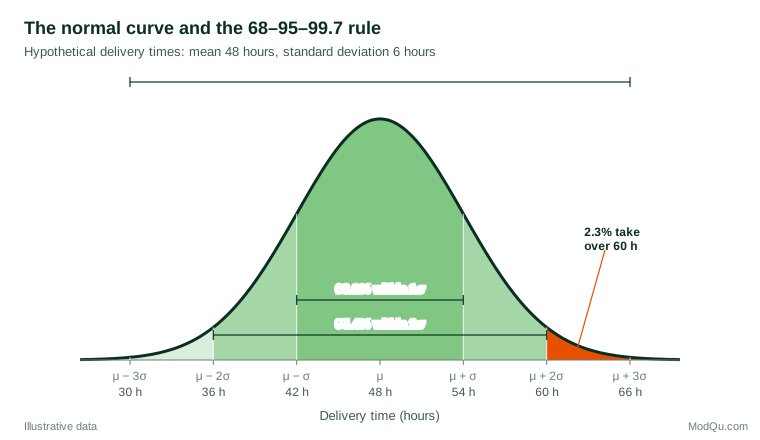
Every normal curve has the same shape once it is rescaled. Converting a value to a z-score, z = (x − μ) ÷ σ, says how many standard deviations it lies from the mean, and the same table of probabilities then applies to any normal variable. This gives the familiar 68–95–99.7 rule: about 68.3% of values fall within one standard deviation of the mean, 95.4% within two, and 99.7% within three.
A worked example
Suppose a hypothetical retailer finds that delivery times for a standard service are approximately normal, with a mean of 48 hours and a standard deviation of 6 hours. How many orders miss a promised 60-hour window? The z-score is (60 − 48) ÷ 6 = 2, and the normal table gives an upper-tail probability of about 2.3%. On 10,000 orders a month, roughly 230 late deliveries can be expected. Promising 54 hours instead (z = 1) would leave about 16% of orders late.
The calculation is quick and useful, but it is only as good as the normality assumption. If delivery times have a long right tail, as many waiting times do, the true share of late orders could be several times larger.
Why it appears everywhere
The main reason is the central limit theorem. When a quantity is the sum or average of many small, roughly independent influences, its distribution tends towards the normal shape, whatever the shape of the individual influences. Mathematicians from de Moivre and Laplace to Lindeberg and Lévy gradually established how general this result is (Fischer, 2011). Measurement errors, heights and many manufacturing tolerances look normal because each is the combined result of many small causes.
Lyon (2014) argues that this explanation is only part of the story. The normal distribution is also the "least informative" distribution for a given mean and variance, so it emerges naturally whenever only those two features are constrained. He also stresses that many quantities described as normal are only approximately so, and only in the middle of the distribution.
For survey and business analysts, the most important application concerns averages, not individuals. Even when individual spending is heavily skewed, the mean spending of a large sample varies from sample to sample in an approximately normal way. That is why margins of error, t-tests and regression coefficients work well in large samples even when the underlying data are far from normal (Lumley et al., 2002).
Where it does not appear
Raw data are a different matter. In a review of 440 large-sample distributions of achievement and psychometric measures, Micceri (1989) found that all of them were significantly non-normal. Blanca et al. (2013) examined 693 small real-data samples and found that only 5.5% came close to normality on both skewness and kurtosis. Common departures in business data include:
- Skewed positive quantities. Income, order values, time on site and company size are bounded at zero and stretched to the right. They are often closer to log-normal, which arises when effects multiply rather than add (Limpert et al., 2001).
- Heavy tails. Price changes and financial returns produce extreme values far more often than a normal curve predicts, a point Mandelbrot (1963) made in his study of cotton prices.
- Bounded and discrete scales. A five-point rating item or a 0–10 recommendation score cannot be truly normal, and responses often pile up at one end.
- Mixtures. Combining distinct customer segments can produce two peaks rather than one.
Checking normality in practice
The most informative check is visual. A normal quantile–quantile (Q–Q) plot places the sorted data against the values a normal distribution would predict; points close to a straight line suggest normality, while curves and bends reveal skewness or heavy tails (Wilk & Gnanadesikan, 1968). Formal tests such as the Shapiro–Wilk test (Shapiro & Wilk, 1965) give a p-value, but their behaviour depends strongly on sample size. In small samples they miss real departures; in the large samples typical of survey work they flag trivial ones. Ghasemi and Zahediasl (2012) therefore recommend combining tests with visual inspection rather than relying on either alone.
Common mistakes
- Assuming raw data are normal and applying the 68–95–99.7 rule to skewed variables such as spend or tenure, which understates extreme values.
- Confusing the data with the estimate. Normality of a sample mean, which large samples usually provide, does not imply normality of the individual responses.
- Over-reacting to normality tests in large samples and abandoning sound methods because of negligible deviations.
- Ignoring the tails. Risk, fraud and service-level questions depend on rare events, where a normal model is least reliable.
Key takeaways
The normal distribution is defined by its mean and standard deviation and gives simple, powerful rules for probabilities. It appears so often because sums and averages of many small effects tend towards it, which is why survey estimates and their margins of error rely on it. Individual business data, however, are usually skewed, bounded or heavy-tailed. Check the shape with a Q–Q plot, transform or model skewed variables appropriately, and reserve normal-based probability statements for quantities that are genuinely close to normal.
References
Blanca, M. J., Arnau, J., López-Montiel, D., Bono, R., & Bendayan, R. (2013). Skewness and kurtosis in real data samples. Methodology, 9(2), 78–84. https://doi.org/10.1027/1614-2241/a000057
Fischer, H. (2011). A history of the central limit theorem: From classical to modern probability theory. Springer. https://doi.org/10.1007/978-0-387-87857-7
Ghasemi, A., & Zahediasl, S. (2012). Normality tests for statistical analysis: A guide for non-statisticians. International Journal of Endocrinology and Metabolism, 10(2), 486–489. https://doi.org/10.5812/ijem.3505
Limpert, E., Stahel, W. A., & Abbt, M. (2001). Log-normal distributions across the sciences: Keys and clues. BioScience, 51(5), 341–352. https://doi.org/10.1641/0006-3568(2001)051[0341:LNDATS]2.0.CO;2
Lumley, T., Diehr, P., Emerson, S., & Chen, L. (2002). The importance of the normality assumption in large public health data sets. Annual Review of Public Health, 23(1), 151–169. https://doi.org/10.1146/annurev.publhealth.23.100901.140546
Lyon, A. (2014). Why are normal distributions normal? The British Journal for the Philosophy of Science, 65(3), 621–649. https://doi.org/10.1093/bjps/axs046
Mandelbrot, B. (1963). The variation of certain speculative prices. The Journal of Business, 36(4), 394–419. https://doi.org/10.1086/294632
Micceri, T. (1989). The unicorn, the normal curve, and other improbable creatures. Psychological Bulletin, 105(1), 156–166. https://doi.org/10.1037/0033-2909.105.1.156
Shapiro, S. S., & Wilk, M. B. (1965). An analysis of variance test for normality (complete samples). Biometrika, 52(3–4), 591–611. https://doi.org/10.1093/biomet/52.3-4.591
Wilk, M. B., & Gnanadesikan, R. (1968). Probability plotting methods for the analysis of data. Biometrika, 55(1), 1–17. https://doi.org/10.1093/biomet/55.1.1