
Statistics · Distributions
Kernel Density Estimation and Nonparametric Distribution Knowledge
How kernel density estimation draws a smooth picture of a distribution without assuming its shape, why the bandwidth matters most, and how to use it well on survey and business data.
Before fitting a model or reporting an average, an analyst needs to know what the data look like. Is customer spending roughly symmetric, skewed, or split into two groups? A kernel density estimate (KDE) answers that question by drawing a smooth curve through the data without assuming any particular shape in advance. The idea goes back to Rosenblatt (1956) and Parzen (1962), and it is now a standard exploratory tool in statistics software and data-visualisation libraries (Silverman, 1986; Scott, 2015).
Why go beyond the histogram?
The histogram is the oldest way to show a distribution, but its picture depends on two arbitrary choices: the bin width and where the first bin starts. Shift the bins by a few units and peaks can appear or vanish. Scott (1979) derived an optimal bin width, which helps, yet a histogram remains a step function that jumps at every bin edge. A parametric alternative, such as fitting a normal distribution, gives a smooth curve but forces the data into a shape chosen before looking. Kernel density estimation sits between the two. It is nonparametric: it lets the data decide the shape, while still producing a smooth, continuous estimate.
How a kernel density estimate works
Place a small, smooth bump (the kernel) on top of every observation, then add up the bumps and rescale so that the total area equals 1. Where observations are crowded, the bumps pile up into a peak; where they are sparse, the curve stays low. Formally, for observations x1, …, xn:
f̂(x) = (1 ÷ nh) × Σi K((x − xi) ÷ h)
Here K is the kernel, usually the bell-shaped normal (Gaussian) curve, and h is the bandwidth, which sets how wide each bump is. Epanechnikov (1969) showed that a parabola-shaped kernel is optimal in a mean squared error sense, but the loss from using another reasonable kernel is small. The choice of kernel matters far less than the choice of bandwidth (Wand & Jones, 1994).
The bandwidth is the key decision
A small bandwidth follows every quirk of the sample and produces a jagged curve with bumps that are mostly noise. A large bandwidth smooths away real features. This is the classic bias–variance trade-off: narrow bumps have low bias but high variance, wide bumps the reverse.
Two families of automatic rules are widely used. Rules of thumb, such as Silverman's (1986) rule, assume the data are roughly normal:
h = 0.9 × min(s, IQR ÷ 1.34) × n−1/5
where s is the standard deviation and IQR the interquartile range. They are quick but tend to oversmooth data with several peaks. Plug-in and cross-validation methods estimate the bandwidth from the data themselves. The plug-in method of Sheather and Jones (1991) performed well in comparative reviews and is a sensible default in most software (Jones et al., 1996; Sheather, 2004). More recent proposals, such as the diffusion-based estimator of Botev et al. (2010), handle strongly multimodal data well.
A worked example
Suppose a hypothetical survey asks 400 households about their weekly grocery spending. The mean is $94 and the median $71. On those figures alone, a report might describe a "typical" household spending somewhere near $90. Figure 1 tells a different story.
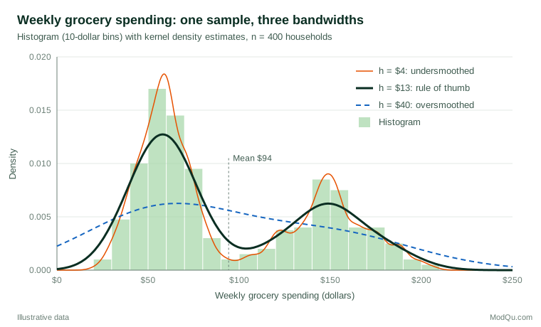
With Silverman's rule (s = 48.4, IQR = 88.3, n = 400), the bandwidth is about $13. The resulting curve shows two clear peaks, one near $58 and one near $149, with a trough near $104. Only about 7% of households spend between $80 and $120, so the mean of $94 describes very few of them. The data look like two segments, perhaps smaller and larger households, and averages should be reported separately for each.
The other two curves show what goes wrong. At $4 the estimate sprouts extra bumps near $122 and $187 that a new sample would not reproduce. At $40 the two segments blur into a single skewed hump, and about 5% of the estimated probability falls below $0, an impossible amount to spend.
Practical guidance for survey and business data
- Always compare a few bandwidths. Plot the automatic choice alongside half and double that value. Features that survive all three are more likely to be real.
- Use weights when the sample is weighted. Each kernel can be multiplied by the respondent's survey weight, so that the curve describes the population rather than the achieved sample.
- Handle boundaries. Spending, time and ages cannot fall below zero, and ratings are capped at both ends. Standard KDE leaks probability past these limits. Boundary corrections, reflection, or estimating on a log scale reduce the problem (Jones, 1993; Chen, 2017).
- Be cautious with rating scales. Five-point or eleven-point answers are discrete. A smooth curve over them can suggest values that nobody chose; a bar chart is often more honest.
- Treat it as exploration, not proof. A bump in a density plot is a hypothesis about a segment. Confirm it with a formal model or a fresh sample.
Limitations and common mistakes
KDE needs more data than a parametric fit to reach the same precision, and the requirement grows quickly with the number of dimensions, so it is most useful for one or two variables at a time (Scott, 2015; Wasserman, 2006). Tails are estimated poorly because few observations fall there; questions about rare extremes call for methods built for tails. Common mistakes include accepting a software default bandwidth without inspection, reading every small wiggle as a segment, ignoring survey weights, and presenting a density plot without saying how the bandwidth was chosen.
Key takeaways
Kernel density estimation gives a smooth, assumption-light picture of a distribution. Its quality depends mainly on the bandwidth, so choose it with a data-based method, check it against narrower and wider alternatives, and respect natural boundaries. Used this way, a density plot can reveal skew, outliers and hidden segments that a mean, a median or a single histogram would miss.
References
Botev, Z. I., Grotowski, J. F., & Kroese, D. P. (2010). Kernel density estimation via diffusion. The Annals of Statistics, 38(5), 2916–2957. https://doi.org/10.1214/10-AOS799
Chen, Y.-C. (2017). A tutorial on kernel density estimation and recent advances. Biostatistics & Epidemiology, 1(1), 161–187. https://doi.org/10.1080/24709360.2017.1396742
Epanechnikov, V. A. (1969). Non-parametric estimation of a multivariate probability density. Theory of Probability & Its Applications, 14(1), 153–158. https://doi.org/10.1137/1114019
Jones, M. C. (1993). Simple boundary correction for kernel density estimation. Statistics and Computing, 3(3), 135–146. https://doi.org/10.1007/BF00147776
Jones, M. C., Marron, J. S., & Sheather, S. J. (1996). A brief survey of bandwidth selection for density estimation. Journal of the American Statistical Association, 91(433), 401–407. https://doi.org/10.1080/01621459.1996.10476701
Parzen, E. (1962). On estimation of a probability density function and mode. The Annals of Mathematical Statistics, 33(3), 1065–1076. https://doi.org/10.1214/aoms/1177704472
Rosenblatt, M. (1956). Remarks on some nonparametric estimates of a density function. The Annals of Mathematical Statistics, 27(3), 832–837. https://doi.org/10.1214/aoms/1177728190
Scott, D. W. (1979). On optimal and data-based histograms. Biometrika, 66(3), 605–610. https://doi.org/10.1093/biomet/66.3.605
Scott, D. W. (2015). Multivariate density estimation: Theory, practice, and visualization (2nd ed.). Wiley. https://doi.org/10.1002/9781118575574
Sheather, S. J. (2004). Density estimation. Statistical Science, 19(4), 588–597. https://doi.org/10.1214/088342304000000297
Sheather, S. J., & Jones, M. C. (1991). A reliable data-based bandwidth selection method for kernel density estimation. Journal of the Royal Statistical Society Series B: Statistical Methodology, 53(3), 683–690. https://doi.org/10.1111/j.2517-6161.1991.tb01857.x
Silverman, B. W. (1986). Density estimation for statistics and data analysis. Chapman and Hall. https://doi.org/10.1201/9781315140919
Wand, M. P., & Jones, M. C. (1994). Kernel smoothing. Chapman and Hall. https://doi.org/10.1201/b14876
Wasserman, L. (2006). All of nonparametric statistics. Springer. https://doi.org/10.1007/0-387-30623-4