
Statistics · Causal inference
Double Machine Learning for Debiased Causal Estimation
How double machine learning uses flexible prediction models to adjust for many confounders while still delivering an unbiased causal estimate with a valid confidence interval, and when it can be trusted.
Modern customer data are wide. A subscription business may hold hundreds of variables on each customer: usage logs, purchase history, survey answers, region and channel. When it asks whether a loyalty programme raises spending, many of those variables are potential confounders, and their relationships with spending and with joining are rarely linear. Ordinary regression with a handful of controls cannot capture them. Machine learning methods such as the lasso, random forests and boosting can, but they are built for prediction, not for estimating a single causal parameter with an honest standard error.
Double machine learning (DML), also called debiased machine learning, bridges this gap. Developed by Chernozhukov et al. (2018), it lets analysts use almost any machine learning method to model the confounders, while the effect of interest is estimated in a way that is approximately unbiased and comes with a valid confidence interval. This article explains why naive approaches fail, how the two ingredients of DML fix them, and how to apply the method sensibly to business and survey data.
The problem: prediction is not estimation
Suppose a customer's annual spend Y depends on whether they joined the loyalty programme, D, and on a large set of characteristics X. A common starting point is the partially linear model:
Y = θD + g(X) + ε and D = m(X) + v
Here θ is the causal effect of interest, g(X) is an unknown and possibly complicated function describing how the characteristics affect spending, and m(X) describes how they affect the chance of joining. If all confounding runs through the measured X, a condition known as unconfoundedness (Rosenbaum & Rubin, 1983), then θ is the average effect of joining.
The difficulty is that g and m are high-dimensional nuisance functions. We do not care about them for their own sake, but θ cannot be estimated well without them. Machine learning methods estimate such functions well in the sense of prediction, yet their estimates are deliberately biased: the lasso shrinks coefficients towards zero (Tibshirani, 1996), and random forests (Breiman, 2001) and gradient boosting (Friedman, 2001) smooth and regularise to avoid overfitting (Hastie et al., 2009). Mullainathan and Spiess (2017) put the distinction well: machine learning is good at producing predictions, not at recovering parameters.
Two things go wrong when a regularised prediction is plugged straight into an estimate of θ:
- Regularisation bias. The deliberate bias in the estimate of g leaks into the estimate of θ. Because machine learning estimates converge more slowly than conventional parametric ones, this bias does not shrink fast enough relative to the standard error, so confidence intervals are centred in the wrong place (Chernozhukov et al., 2018).
- Overfitting bias. If the same observations are used to fit g and to estimate θ, the model's fit to noise in those observations distorts the estimate.
A related trap is to select controls with a variable-selection method and then run ordinary regression as if the selected model had been fixed in advance. Leeb and Pötscher (2005) showed that inference after data-driven model selection can be badly misleading. Belloni et al. (2014a) illustrated a specific failure: a lasso of the outcome on the controls may drop a confounder that is only weakly related to the outcome but strongly related to treatment, leaving substantial omitted variable bias.
Partialling out: an old idea
The solution builds on a classical result. In linear regression, the coefficient on D from a regression of Y on D and X equals the coefficient from regressing the part of Y not explained by X on the part of D not explained by X. This is the Frisch–Waugh theorem (Frisch & Waugh, 1933). Robinson (1988) extended the idea to the partially linear model with a nonparametric g, showing that θ can be estimated at the usual rate by regressing residuals on residuals:
θ̂ = Σi (Di − m̂(Xi))(Yi − ℓ̂(Xi)) ÷ Σi (Di − m̂(Xi))2
where ℓ(X) is the expected outcome given X and m(X) is the expected treatment given X. Two prediction problems, predicting the outcome and predicting the treatment, give the method its name.
Ingredient 1: Neyman orthogonality
Why does residualising both variables help? The residual-on-residual estimator is built on a Neyman-orthogonal score: its expected value is insensitive to small errors in the nuisance functions. Errors in ℓ̂ and in m̂ enter the estimate of θ only through their product. If each nuisance estimate is moderately accurate, their product is small, and the estimate of θ behaves as if the nuisance functions had been known (Chernozhukov et al., 2018). Semiparametric theory explains why estimators built on such scores are not affected, to first order, by the estimation of the nuisance functions (Newey, 1994).
By contrast, an estimator that adjusts only the outcome, by subtracting ĝ(X) from Y and regressing the result on D, has a first-order sensitivity to errors in ĝ. That is where regularisation bias comes from.
The same principle underlies doubly robust estimation. The augmented inverse probability weighting estimator of the average treatment effect, introduced by Robins et al. (1994) and explained accessibly by Bang and Robins (2005), combines an outcome model with a propensity score model. Its score is:
ψ = μ̂1(X) − μ̂0(X) + D(Y − μ̂1(X)) ÷ ê(X) − (1 − D)(Y − μ̂0(X)) ÷ (1 − ê(X))
where μ̂1 and μ̂0 predict the outcome with and without treatment and ê(X) is the estimated propensity score. The average of ψ is consistent if either model is correct, and it is Neyman-orthogonal, so DML uses it for binary treatments. Targeted maximum likelihood estimation reaches similar properties by a different route (van der Laan & Rubin, 2006).
Ingredient 2: cross-fitting
Orthogonality deals with regularisation bias. Overfitting bias is handled by cross-fitting, shown in Figure 1. The sample is split into K folds, often five. For each fold, the nuisance models are trained on the other folds and used to compute residuals for the held-out fold. Every observation's residual therefore comes from models that never saw it. The residuals from all folds are pooled to estimate θ and its standard error.
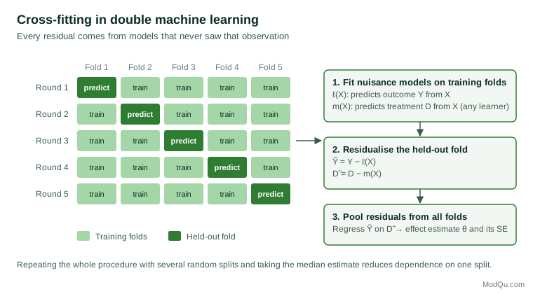
Unlike simple sample splitting, cross-fitting uses every observation for the final estimate, so there is no loss of efficiency. Because results depend somewhat on the random split, Chernozhukov et al. (2018) recommend repeating the procedure with several splits and aggregating the results, for example by taking the median. Zivich and Breskin (2021) found in simulations that doubly robust estimators combined with flexible machine learning gave confidence intervals with close to nominal coverage when cross-fitting was used, and markedly worse coverage without it.
What the method buys: a simulation
Figure 2 shows a small simulation in the spirit of those reported by Chernozhukov et al. (2018). Data were generated from a partially linear model with ten correlated covariates, nonlinear nuisance functions and a true effect of θ = 0.5, with 500 observations per sample. Random forests were used for every nuisance model. A naive plug-in estimator, which uses the forest to adjust only the outcome, gave estimates averaging 0.44 across 300 simulated samples, biased downwards by about 13% of the true effect and by roughly one standard deviation of its own sampling distribution. The DML estimator, with orthogonal residualising and two-fold cross-fitting, averaged 0.49, close to the truth. Its nominal 95% confidence interval contained the true value in 90% of samples: much better than intervals centred on a biased estimate, but a little below the nominal level, a reminder that the guarantees are large-sample results and that modest samples, few folds and a single split all leave some residual error.
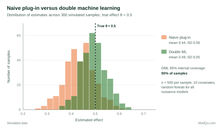
Both estimators used the same flexible learner. The difference lies entirely in how the learner's output was used.
A worked example
Consider a hypothetical retailer with records on 20,000 customers, of whom 6,000 joined a loyalty programme last year. For each customer it holds 180 pre-programme variables: spending by category over the previous two years, visit frequency, channel use, demographics and answers to an annual satisfaction survey. Members spent on average $640 more than non-members in the following year, but members were already heavier spenders before joining.
Three illustrative analyses give different answers:
| Method | Estimated effect on annual spend | 95% interval |
|---|---|---|
| Raw difference in means | $640 | $610 to $670 |
| Linear regression with 8 hand-picked controls | $310 | $270 to $350 |
| Double machine learning (gradient boosting, 5 folds, 10 repeated splits) | $185 | $135 to $235 |
The DML estimate adjusts for all 180 variables, including nonlinear patterns such as a sharp rise in membership among customers whose spending was climbing just before the programme launched. The hand-picked regression misses those patterns and attributes some pre-existing momentum to the programme. In this example, the decision to expand the programme would look very different at $185 per member than at $640.
Two checks support the result. The estimated propensity scores range from 0.04 to 0.93, so treated and untreated customers overlap across the range of characteristics. And the estimate changes little when the gradient boosting models are replaced by the lasso or random forests, which suggests that it does not depend on one learner's quirks.
Where DML fits among causal methods
The same recipe extends well beyond the partially linear model. Chernozhukov et al. (2018) apply it to average treatment effects with a binary treatment, to effects among the treated, and to instrumental variable models in which an instrument shifts treatment, using the appropriate orthogonal score in each case. The post-double-selection lasso of Belloni et al. (2014a), which keeps every control selected by a lasso of either the outcome or the treatment, can be seen as an early special case: it guards against the omitted-confounder problem by modelling both relationships.
Compared with propensity score matching or weighting, DML uses the outcome model as well as the treatment model, which typically improves precision and gives some protection if one of them is misspecified. Compared with a conventional regression, it removes the need to guess functional forms for dozens of controls. What it shares with all of these methods is the identifying assumption: it estimates a causal effect only if the measured covariates capture the reasons why some customers were treated and others were not.
Practical guidance for survey and business data
- Start from a causal design. DML adjusts for measured confounders more flexibly than regression. It does nothing about unmeasured ones. Decide which variables are pre-treatment confounders before modelling, and leave out anything the treatment could affect.
- Check overlap. Examine the distribution of estimated propensity scores. Scores near 0 or 1 make the doubly robust score unstable; trimming the sample or changing the estimand to the effect among the treated may be necessary.
- Use good learners and compare them. The guarantees require nuisance estimates that are reasonably accurate. Compare out-of-fold prediction error across learners or use an ensemble, and report whether θ̂ is stable across them.
- Repeat the splits. Report the median over several random splits and the variation across them.
- Respect the survey design. With weighted survey data or clustered samples, carry the weights through the final estimation step and use clustered or design-based standard errors. Assign whole clusters, such as households or stores, to the same fold so that information does not leak between folds.
- Run a sensitivity analysis. Quantify how strong an unmeasured confounder would need to be to change the conclusion (Cinelli & Hazlett, 2020).
- Use tested software. Open-source implementations such as DoubleML handle cross-fitting, repeated splits and standard errors consistently (Bach et al., 2022).
Common mistakes
- Believing that more variables means no confounding. Hundreds of controls do not guarantee that the key confounder was measured.
- Including post-treatment variables. Satisfaction measured after joining, or spending in the months after the programme started, absorbs part of the effect and biases the estimate.
- Skipping cross-fitting because the learner seems not to overfit. The theory requires it, and simulations show poor interval coverage without it.
- Interpreting feature importance as causal. The nuisance models are prediction devices; their internal structure says nothing about what causes what.
- Treating θ as a constant. The partially linear model estimates one average effect. If effects vary across customers, methods for heterogeneous effects are needed.
Key takeaways
Double machine learning lets analysts use flexible prediction methods to adjust for many confounders without giving up valid inference on the causal effect. It works by combining a Neyman-orthogonal score, which makes the estimate insensitive to small errors in the prediction models, with cross-fitting, which prevents overfitting from leaking into the estimate. Its guarantees rest on unconfoundedness, overlap and reasonably accurate nuisance models. Used with careful design, overlap checks and sensitivity analysis, it is one of the most useful tools for causal questions in wide observational data (Athey & Imbens, 2019; Belloni et al., 2014b; Chernozhukov et al., 2017).
References
Athey, S., & Imbens, G. W. (2019). Machine learning methods that economists should know about. Annual Review of Economics, 11, 685–725. https://doi.org/10.1146/annurev-economics-080217-053433
Bach, P., Chernozhukov, V., Kurz, M. S., & Spindler, M. (2022). DoubleML: An object-oriented implementation of double machine learning in Python. Journal of Machine Learning Research, 23(53), 1–6.
Bang, H., & Robins, J. M. (2005). Doubly robust estimation in missing data and causal inference models. Biometrics, 61(4), 962–973. https://doi.org/10.1111/j.1541-0420.2005.00377.x
Belloni, A., Chernozhukov, V., & Hansen, C. (2014a). Inference on treatment effects after selection among high-dimensional controls. The Review of Economic Studies, 81(2), 608–650. https://doi.org/10.1093/restud/rdt044
Belloni, A., Chernozhukov, V., & Hansen, C. (2014b). High-dimensional methods and inference on structural and treatment effects. Journal of Economic Perspectives, 28(2), 29–50. https://doi.org/10.1257/jep.28.2.29
Breiman, L. (2001). Random forests. Machine Learning, 45(1), 5–32. https://doi.org/10.1023/A:1010933404324
Chernozhukov, V., Chetverikov, D., Demirer, M., Duflo, E., Hansen, C., & Newey, W. (2017). Double/debiased/Neyman machine learning of treatment effects. American Economic Review, 107(5), 261–265. https://doi.org/10.1257/aer.p20171038
Chernozhukov, V., Chetverikov, D., Demirer, M., Duflo, E., Hansen, C., Newey, W., & Robins, J. (2018). Double/debiased machine learning for treatment and structural parameters. The Econometrics Journal, 21(1), C1–C68. https://doi.org/10.1111/ectj.12097
Cinelli, C., & Hazlett, C. (2020). Making sense of sensitivity: Extending omitted variable bias. Journal of the Royal Statistical Society Series B: Statistical Methodology, 82(1), 39–67. https://doi.org/10.1111/rssb.12348
Friedman, J. H. (2001). Greedy function approximation: A gradient boosting machine. The Annals of Statistics, 29(5), 1189–1232. https://doi.org/10.1214/aos/1013203451
Frisch, R., & Waugh, F. V. (1933). Partial time regressions as compared with individual trends. Econometrica, 1(4), 387–401. https://doi.org/10.2307/1907330
Hastie, T., Tibshirani, R., & Friedman, J. (2009). The elements of statistical learning: Data mining, inference, and prediction (2nd ed.). Springer. https://doi.org/10.1007/978-0-387-84858-7
Leeb, H., & Pötscher, B. M. (2005). Model selection and inference: Facts and fiction. Econometric Theory, 21(1), 21–59. https://doi.org/10.1017/S0266466605050036
Mullainathan, S., & Spiess, J. (2017). Machine learning: An applied econometric approach. Journal of Economic Perspectives, 31(2), 87–106. https://doi.org/10.1257/jep.31.2.87
Newey, W. K. (1994). The asymptotic variance of semiparametric estimators. Econometrica, 62(6), 1349–1382. https://doi.org/10.2307/2951752
Robins, J. M., Rotnitzky, A., & Zhao, L. P. (1994). Estimation of regression coefficients when some regressors are not always observed. Journal of the American Statistical Association, 89(427), 846–866. https://doi.org/10.1080/01621459.1994.10476818
Robinson, P. M. (1988). Root-N-consistent semiparametric regression. Econometrica, 56(4), 931–954. https://doi.org/10.2307/1912705
Rosenbaum, P. R., & Rubin, D. B. (1983). The central role of the propensity score in observational studies for causal effects. Biometrika, 70(1), 41–55. https://doi.org/10.1093/biomet/70.1.41
Tibshirani, R. (1996). Regression shrinkage and selection via the lasso. Journal of the Royal Statistical Society Series B: Statistical Methodology, 58(1), 267–288. https://doi.org/10.1111/j.2517-6161.1996.tb02080.x
van der Laan, M. J., & Rubin, D. (2006). Targeted maximum likelihood learning. The International Journal of Biostatistics, 2(1), Article 11. https://doi.org/10.2202/1557-4679.1043
Zivich, P. N., & Breskin, A. (2021). Machine learning for causal inference: On the use of cross-fit estimators. Epidemiology, 32(3), 393–401. https://doi.org/10.1097/EDE.0000000000001332