
Statistics · Distributions
Binomial and Poisson Distributions in Business Applications
How the binomial and Poisson distributions describe yes/no outcomes and event counts, with worked business examples, the link between them, and the mistakes that most often mislead analysts.
A great deal of business data is counted rather than measured. How many of 20 prospects accepted an offer? How many survey respondents said they would switch brands? How many complaints arrived today, or how many calls in the next quarter hour? Two probability distributions sit behind most of these questions. The binomial distribution describes the number of "successes" in a fixed number of yes/no trials. The Poisson distribution describes the number of events in a fixed interval of time or space when events occur independently at a steady average rate. Both are among the oldest models in statistics, and both remain everyday tools in market research, operations and quality management (Johnson et al., 2005).
The binomial distribution
The binomial distribution goes back to Jacob Bernoulli's Ars Conjectandi, published in 1713, which studied repeated trials with two possible outcomes (Bernoulli, 2006; Stigler, 1986). It applies when four conditions hold:
- There is a fixed number of trials, n.
- Each trial has only two outcomes, conventionally called success and failure.
- The probability of success, p, is the same on every trial.
- The trials are independent of one another.
The probability of exactly k successes is:
P(X = k) = C(n, k) × pk × (1 − p)n − k
where C(n, k) is the number of ways of choosing k items from n. The mean is np and the variance is np(1 − p). The variance is largest when p = 0.5 and shrinks as p approaches 0 or 1, which is why survey percentages near 50% carry the widest margins of error.
Worked example: a sales campaign
Suppose, hypothetically, that a sales team contacts 20 qualified prospects and each converts independently with probability 0.15. The expected number of conversions is 20 × 0.15 = 3, with a standard deviation of √(20 × 0.15 × 0.85) ≈ 1.6. The binomial formula gives further useful answers:
- The chance of no conversions at all is 0.8520 ≈ 3.9%.
- The chance of one or fewer is about 17.6%.
- The chance of five or more is about 17.0%.
So a week with only one sale, or a week with five, is not unusual under an unchanged 15% conversion rate. A manager who praises or blames the team on the strength of such swings is reacting to chance. The binomial distribution gives a baseline against which genuinely unusual results can be judged.
Binomial counts in surveys
Every percentage in a survey report is, in effect, a binomial count divided by the sample size. If 30% of 400 randomly sampled respondents say they would buy a new product, the standard error of that percentage is √(0.30 × 0.70 ÷ 400) ≈ 2.3 percentage points, and the familiar 95% margin of error is about ±4.5 points. This simple formula assumes a simple random sample. Weighting, clustering and stratification change the variance, and design-based methods are needed to estimate it properly (Lohr, 2021).
The textbook "Wald" interval, p ± 1.96 × standard error, also behaves poorly when samples are small or percentages are near 0% or 100%. Brown et al. (2001) showed that its actual coverage can fall well below 95% even for moderately large samples. For 2 conversions out of 25 trials, the Wald interval runs from −2.6% to 18.6%, an impossible negative lower limit. The interval proposed by Wilson (1927) runs from 2.2% to 25.0%, which is both possible and more accurate. Agresti and Coull (1998) recommend Wilson-type intervals, or the simple adjusted interval that adds two successes and two failures, over both the Wald and the conservative "exact" interval of Clopper and Pearson (1934).
The Poisson distribution
The Poisson distribution is named after Siméon-Denis Poisson, who derived it in 1837 as a limiting case of the binomial (Stigler, 1986). It became famous through Bortkiewicz (1898), who showed that rare events such as deaths from horse kicks in Prussian army corps followed it closely. The distribution applies when events occur one at a time, independently of one another, at a constant average rate λ (lambda) per interval. The probability of exactly k events in an interval is:
P(X = k) = e−λ × λk ÷ k!
A distinctive property is that the mean and the variance are both equal to λ. This makes the Poisson distribution easy to check: if the variance of observed counts is much larger than their mean, the simple model does not fit.
Worked example: complaints and call arrivals
Suppose, hypothetically, that a retailer receives an average of 3 customer complaints per day. Under a Poisson model:
- The chance of a complaint-free day is e−3 ≈ 5.0%.
- The chance of five or fewer complaints is about 91.6%.
- The chance of seven or more is about 3.4%.
A day with seven complaints is therefore a reasonable trigger for investigation, because it would occur by chance only about once a month. This is the logic of the c-chart used in statistical process control to monitor counts of defects or incidents.
The same reasoning supports staffing decisions. If a contact centre receives an average of 4 calls per 15 minutes, the Poisson distribution shows that 6 or fewer calls will arrive in about 89% of intervals and 8 or fewer in about 98%. Poisson arrivals are the starting point of the queueing models used to plan contact centre capacity, although real arrival rates vary through the day and must be forecast interval by interval (Gans et al., 2003).
How the two distributions are related
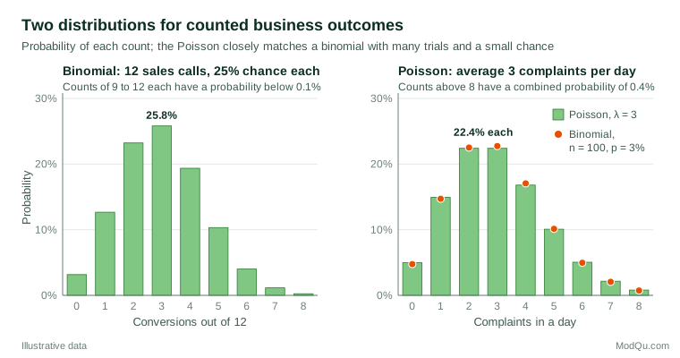
When the number of trials is large and the probability of success is small, the binomial distribution with n trials and probability p is very close to a Poisson distribution with λ = np. Figure 1 shows the binomial with 100 trials and a 3% chance alongside the Poisson with λ = 3: no single probability differs by more than about a third of a percentage point. Le Cam (1960) gave a precise bound on the error of this approximation, which holds even when the success probabilities differ from trial to trial: the total error is no more than twice the sum of the squared probabilities. In practice the approximation is excellent for rare events such as product returns, fraud cases or insurance claims within a large customer base, where the exact number of "trials" may not even be known (Blitzstein & Hwang, 2019).
Practical guidance for business and survey data
- Choose the model from the data-generating process. Use the binomial when there is a known number of trials and each can succeed or fail, such as respondents, emails sent or units inspected. Use the Poisson when you count events in an interval with no natural upper limit, such as calls, visits, claims or defects.
- Use better intervals for proportions. For small samples or rare outcomes, report Wilson or Agresti–Coull intervals rather than the Wald interval (Brown et al., 2001).
- Use the rule of three for zero events. If none of n independent trials fails, an approximate 95% upper confidence limit for the failure rate is 3 ÷ n (Hanley & Lippman-Hand, 1983). Zero defects in 300 inspected units still allows a true defect rate of up to about 1%.
- Plan experiments with binomial variance in mind. Conversion rates in online experiments are binomial, and detecting a small change in a low base rate requires very large samples (Kohavi et al., 2020).
- Check the mean–variance relationship. Before relying on a Poisson model, compare the variance of the observed counts with their mean. A ratio close to 1 supports the model; a ratio well above 1 signals that the counts are clustered or that customers differ in their underlying rates.
- Model counts with count models. When counts depend on predictors, such as visits by customer segment, Poisson regression and its extensions are more suitable than ordinary linear regression (Cameron & Trivedi, 2013).
Common mistakes
- Ignoring overdispersion. Real counts are often more variable than the Poisson allows, because customers differ in their underlying rates. Ehrenberg (1959) showed that purchase frequencies across consumers are better described by the negative binomial distribution, a Poisson whose rate varies from person to person. Treating overdispersed data as Poisson understates uncertainty and produces false alarms; the negative binomial model is the usual remedy (Hilbe, 2011).
- Overlooking excess zeros. Many customers never complain, never claim and never return a product. When there are more zeros than either model predicts, zero-inflated models separate the "never" group from the rest (Lambert, 1992).
- Assuming independence that is not there. Complaints often arrive in bursts after a single service failure, and respondents in the same household or branch tend to answer alike. Such dependence widens the true variability beyond the binomial or Poisson value.
- Assuming a constant rate or probability. Calls peak at lunchtime and conversion rates differ by channel. Pooling intervals or groups with different rates produces a misleading single average.
Key takeaways
The binomial distribution describes successes in a fixed number of yes/no trials and underlies every survey percentage, conversion rate and pass/fail inspection. The Poisson distribution describes counts of independent events at a steady rate and underlies arrivals, complaints, claims and defects. The two are closely linked, since the Poisson is the limit of the binomial for many trials with a small chance of success. Both give a valuable baseline for separating real change from chance, but both rest on assumptions of independence and constant rates. Check those assumptions, use good intervals for proportions, and turn to negative binomial or zero-inflated models when the data are more variable than the simple models allow.
References
Agresti, A., & Coull, B. A. (1998). Approximate is better than "exact" for interval estimation of binomial proportions. The American Statistician, 52(2), 119–126. https://doi.org/10.1080/00031305.1998.10480550
Bernoulli, J. (2006). The art of conjecturing, together with Letter to a friend on sets in court tennis (E. D. Sylla, Trans.). Johns Hopkins University Press. (Original work published 1713)
Blitzstein, J. K., & Hwang, J. (2019). Introduction to probability (2nd ed.). Chapman and Hall/CRC. https://doi.org/10.1201/9780429428357
Bortkiewicz, L. von. (1898). Das Gesetz der kleinen Zahlen. B. G. Teubner.
Brown, L. D., Cai, T. T., & DasGupta, A. (2001). Interval estimation for a binomial proportion. Statistical Science, 16(2), 101–133. https://doi.org/10.1214/ss/1009213286
Cameron, A. C., & Trivedi, P. K. (2013). Regression analysis of count data (2nd ed.). Cambridge University Press. https://doi.org/10.1017/CBO9781139013567
Clopper, C. J., & Pearson, E. S. (1934). The use of confidence or fiducial limits illustrated in the case of the binomial. Biometrika, 26(4), 404–413. https://doi.org/10.1093/biomet/26.4.404
Ehrenberg, A. S. C. (1959). The pattern of consumer purchases. Journal of the Royal Statistical Society: Series C (Applied Statistics), 8(1), 26–41. https://doi.org/10.2307/2985810
Gans, N., Koole, G., & Mandelbaum, A. (2003). Telephone call centers: Tutorial, review, and research prospects. Manufacturing & Service Operations Management, 5(2), 79–141. https://doi.org/10.1287/msom.5.2.79.16071
Hanley, J. A., & Lippman-Hand, A. (1983). If nothing goes wrong, is everything all right? Interpreting zero numerators. JAMA, 249(13), 1743–1745. https://doi.org/10.1001/jama.1983.03330370053031
Hilbe, J. M. (2011). Negative binomial regression (2nd ed.). Cambridge University Press. https://doi.org/10.1017/CBO9780511973420
Johnson, N. L., Kemp, A. W., & Kotz, S. (2005). Univariate discrete distributions (3rd ed.). Wiley. https://doi.org/10.1002/0471715816
Kohavi, R., Tang, D., & Xu, Y. (2020). Trustworthy online controlled experiments: A practical guide to A/B testing. Cambridge University Press. https://doi.org/10.1017/9781108653985
Lambert, D. (1992). Zero-inflated Poisson regression, with an application to defects in manufacturing. Technometrics, 34(1), 1–14. https://doi.org/10.2307/1269547
Le Cam, L. (1960). An approximation theorem for the Poisson binomial distribution. Pacific Journal of Mathematics, 10(4), 1181–1197. https://doi.org/10.2140/pjm.1960.10.1181
Lohr, S. L. (2021). Sampling: Design and analysis (3rd ed.). Chapman and Hall/CRC. https://doi.org/10.1201/9780429298899
Stigler, S. M. (1986). The history of statistics: The measurement of uncertainty before 1900. Belknap Press of Harvard University Press.
Wilson, E. B. (1927). Probable inference, the law of succession, and statistical inference. Journal of the American Statistical Association, 22(158), 209–212. https://doi.org/10.1080/01621459.1927.10502953