
Statistics · Communication and misuse
Base Rate Neglect and the Misreading of Probabilities
Why accurate tests, models and screeners still produce mostly false alarms when the thing they look for is rare, how to correct the reasoning with Bayes' theorem, and how to present probabilities so they are understood.
A fraud model is described as 95% accurate. It flags a transaction. What is the chance that the transaction is actually fraudulent? Most people, including many analysts, answer "about 95%". The true answer may be nearer 25%. The gap comes from ignoring how common fraud is in the first place. This error, base rate neglect, is one of the best documented mistakes in probabilistic reasoning, and it affects medical testing, fraud detection, survey screening, predictive models and the reading of significance tests alike.
What base rate neglect is
The base rate is the proportion of cases in the relevant population that have the characteristic of interest before any specific evidence is considered: the share of transactions that are fraudulent, of customers who will cancel, or of respondents who truly belong to a target group. Base rate neglect is the tendency to judge the probability of an outcome from the specific evidence alone, giving the base rate too little weight or none.
The classic demonstrations come from Kahneman and Tversky (1973). Participants read short personality descriptions said to be drawn from a group of engineers and lawyers. Some were told the group contained 30 engineers and 70 lawyers; others were told the reverse. Their judgments of whether a description belonged to an engineer barely changed with these proportions. People judged by how well the description matched a stereotype, a strategy Tversky and Kahneman (1974) called the representativeness heuristic, and largely ignored the prior probabilities. In the related taxicab problem analysed by Bar-Hillel (1980), 85% of a city's cabs are green and 15% blue, and a witness who is right 80% of the time says the cab in an accident was blue. Most people put the probability that it was blue close to 80%, when the correct answer is about 41%.
The arithmetic: Bayes' theorem
The correct combination of a base rate with new evidence is given by Bayes' theorem (Bayes, 1763). For a condition C and a positive result +:
P(C | +) = P(+ | C) × P(C) ÷ [P(+ | C) × P(C) + P(+ | not C) × P(not C)]
Here P(C) is the base rate, P(+ | C) is the sensitivity (the share of true cases that are detected) and P(+ | not C) is the false positive rate, equal to one minus the specificity. The result, P(C | +), is the positive predictive value: the share of positive results that are correct. A form that is easier to use mentally works with odds:
Posterior odds = prior odds × likelihood ratio
where the likelihood ratio for a positive result is the sensitivity divided by the false positive rate. The formula makes the central point plain. However strong the evidence, a very low prior odds can still leave a low posterior probability.
A worked example: screening for fraud
Consider a hypothetical card issuer. Of every 1,000 transactions, 20 are fraudulent, a base rate of 2%. Its screening model detects 90% of frauds and wrongly flags 5% of genuine transactions. Figure 1 shows what happens to 1,000 transactions.
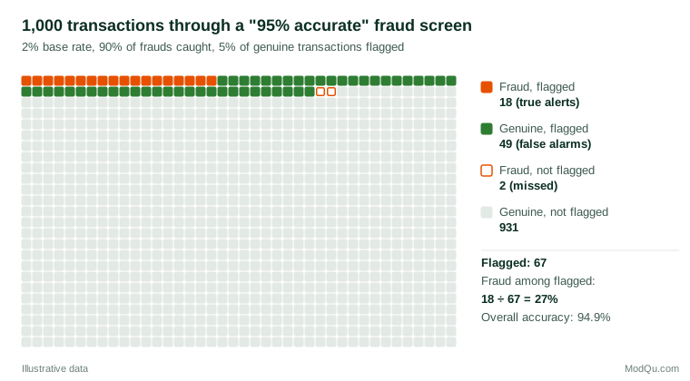
The model catches 18 of the 20 frauds but also flags 49 of the 980 genuine transactions. Of the 67 flagged, only 18 are fraud, a positive predictive value of 27%. In odds form, the prior odds are 20 to 980, about 0.02, and the likelihood ratio is 0.90 ÷ 0.05 = 18, giving posterior odds of about 0.37, or a probability of 27%. The model is useful, since a flagged transaction is about 13 times more likely to be fraud than a random one, but most alerts are still false. Its headline accuracy of 94.9% says little: a rule that flagged nothing at all would score 98%.
How the base rate drives the answer
Figure 2 shows the positive predictive value of three hypothetical tests across base rates from 0.1% to 50%. The same test can be highly informative in one population and nearly useless in another. A test with 90% sensitivity and 90% specificity gives a predictive value of 8% when the base rate is 1%, but 90% when it is 50%. Even a test with 99% sensitivity and 99.9% specificity, far better than most business models, is right only half the time when the base rate is 0.1%.
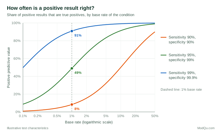
This is why predictive values cannot be carried from one setting to another without adjusting for prevalence (Altman & Bland, 1994). A model validated on a balanced sample, or on a segment where churn is common, will produce far more false alarms when deployed across the whole customer base.
Experts make the same mistake
Base rate neglect is not confined to untrained people. Casscells et al. (1978) asked staff and students at a medical school a simple question: if a disease has a prevalence of 1 in 1,000 and a test has a false positive rate of 5%, what is the chance that a person with a positive result has the disease? Only 11 of the 60 participants gave the correct answer of about 2%, and the most common answer was 95%. Later studies with physicians found similar confusion when test results were presented as conditional probabilities (Gigerenzer et al., 2007).
The error has a name in the courtroom. The prosecutor's fallacy treats the probability of the evidence given innocence, such as a one-in-a-million chance of a random match, as if it were the probability of innocence given the evidence. Thompson and Schumann (1987) showed that mock jurors were vulnerable both to this error and to its mirror image, the defence attorney's fallacy, which dismisses strong evidence by pointing to the number of people in a large population who might also match.
Why people neglect base rates
Several explanations have been offered, and they are not mutually exclusive.
- Representativeness. Specific, vivid evidence feels more relevant than an abstract statistic about a population (Tversky & Kahneman, 1974).
- Confusing conditional probabilities. The probability of a positive result given the condition is easily mistaken for the probability of the condition given a positive result. The two are equal only when the base rate and the overall positive rate are the same.
- Presentation format. Gigerenzer and Hoffrage (1995) found that when the same information was presented as natural frequencies ("10 of every 1,000 women have the disease; 8 of those 10 test positive"), the share of correct Bayesian answers rose from 16% to 46% across their problems. Cosmides and Tooby (1996) reported similar gains and argued that the mind handles frequencies of events more easily than single-event probabilities. A meta-analysis by McDowell and Jacobs (2017) confirmed that natural frequencies improve performance, although many people still err.
- Perceived relevance. Koehler (1996) reviewed the literature and argued that base rates are not always ignored. People use them more when they appear causally relevant, when they are clearly drawn from the population in question and when the task makes them salient. In real decisions it is also not always obvious which reference population supplies the right base rate.
Where base rates matter in business and research
Fraud, risk and anomaly detection
Fraud and security problems combine very low base rates with large volumes of data. Bolton and Hand (2002) noted that the rarity of fraud means even small false positive rates generate many more false alarms than genuine cases. Axelsson (2000) applied the same reasoning to computer intrusion detection and concluded that a useful system must keep its false alarm rate extremely low, because intrusions are rare compared with normal events. For these tasks overall accuracy and the ROC curve can look excellent while most alerts are wrong. Saito and Rehmsmeier (2015) showed that precision-recall plots, which incorporate the base rate, give a more informative picture than ROC plots for such imbalanced data.
Survey screeners and low-incidence groups
Market research often needs respondents from small groups, such as owners of a niche product. Suppose 3% of a sample truly own the product, a screener question admits 95% of owners, and 2% of non-owners pass by mistake, through misreading or overclaiming. Per 10,000 people screened, 285 true owners qualify and 194 non-owners also qualify, so about 40% of the "qualified" sample does not belong to the target group. The rarer the group, the more a small error rate in screening contaminates the results. Validation questions and checks on implausible answers matter most when incidence is low.
Targeting and predictive models
Lead scores, churn models and propensity scores are often summarised by sensitivity or lift on a test file. Whether acting on a score is worthwhile depends on the base rate in the population where it will be applied and on the costs of false alarms and misses. Reporting the expected number of true and false positives per 1,000 customers makes the trade-off visible to decision-makers, who can then judge whether the cost of contacting the false positives is worth the value of reaching the true ones.
Significance tests and research findings
A p-value is the probability of data at least as extreme as those observed if the null hypothesis is true. It is not the probability that the null hypothesis is true (Wasserstein & Lazar, 2016). Reading it that way is a form of base rate neglect, because the probability that an effect is real also depends on how many of the hypotheses being tested are true. Colquhoun (2014) showed that if 10% of tested hypotheses are true and studies have 80% power, about 36% of results significant at the 5% level are false positives. Ioannidis (2005) used the same logic to argue that, in fields with low prior odds, small studies and flexible analyses, most published positive findings may be false. Testing many speculative ideas, such as dozens of campaign variants, lowers the base rate of real effects and should raise the bar for believing any single "win".
Communicating probabilities so they are understood
- State the reference population. "27% of flagged transactions are fraud" is clearer than "the model is 90% sensitive", and both are clearer than an unlabelled "accuracy".
- Use natural frequencies. Express results as counts out of a round number, such as 18 of 67 alerts per 1,000 transactions (Gigerenzer & Hoffrage, 1995; Hoffrage et al., 2000).
- Show icon arrays or frequency grids. Pictures of whole populations, such as Figure 1, help people with lower numeracy understand risk (Galesic et al., 2009) and are widely recommended for communicating uncertainty (Spiegelhalter et al., 2011).
- Report predictive values for the relevant base rate. If a model will be used in several segments, show how its precision changes between them, as in Figure 2.
- Give absolute as well as relative figures. "Ten times more likely" sounds dramatic, but from a base of 1 in 10,000 it still means 1 in 1,000 (Gigerenzer et al., 2007).
Common mistakes
- Quoting accuracy for rare outcomes. With a 2% base rate, a model that predicts "no" for everyone is 98% accurate.
- Reading P(evidence | hypothesis) as P(hypothesis | evidence). This is the core of both the prosecutor's fallacy and the misreading of p-values.
- Transferring predictive values between populations. A screen that works in a high-risk segment can fail across the whole market.
- Ignoring how many hypotheses were tried. The more ideas tested, the lower the base rate of true effects among those that reach significance.
- Treating the base rate as fixed. Fraud rates, churn rates and incidence change over time and between segments, and estimates of them should be updated.
Key takeaways
The meaning of any positive result depends on how common the condition was before the result arrived. Sensitivity, specificity and accuracy describe a test or model; only the base rate turns them into the probability that a particular alert, respondent or finding is genuine. When the outcome is rare, most positives can be false even for a good test. Combine evidence with Bayes' theorem, report results as natural frequencies for a stated population, and be most sceptical where base rates are lowest.
References
Altman, D. G., & Bland, J. M. (1994). Diagnostic tests 2: Predictive values. BMJ, 309(6947), 102. https://doi.org/10.1136/bmj.309.6947.102
Axelsson, S. (2000). The base-rate fallacy and the difficulty of intrusion detection. ACM Transactions on Information and System Security, 3(3), 186–205. https://doi.org/10.1145/357830.357849
Bar-Hillel, M. (1980). The base-rate fallacy in probability judgments. Acta Psychologica, 44(3), 211–233. https://doi.org/10.1016/0001-6918(80)90046-3
Bayes, T. (1763). An essay towards solving a problem in the doctrine of chances. Philosophical Transactions of the Royal Society of London, 53, 370–418. https://doi.org/10.1098/rstl.1763.0053
Bolton, R. J., & Hand, D. J. (2002). Statistical fraud detection: A review. Statistical Science, 17(3), 235–255. https://doi.org/10.1214/ss/1042727940
Casscells, W., Schoenberger, A., & Graboys, T. B. (1978). Interpretation by physicians of clinical laboratory results. New England Journal of Medicine, 299(18), 999–1001. https://doi.org/10.1056/NEJM197811022991808
Colquhoun, D. (2014). An investigation of the false discovery rate and the misinterpretation of p-values. Royal Society Open Science, 1(3), Article 140216. https://doi.org/10.1098/rsos.140216
Cosmides, L., & Tooby, J. (1996). Are humans good intuitive statisticians after all? Rethinking some conclusions from the literature on judgment under uncertainty. Cognition, 58(1), 1–73. https://doi.org/10.1016/0010-0277(95)00664-8
Galesic, M., Garcia-Retamero, R., & Gigerenzer, G. (2009). Using icon arrays to communicate medical risks: Overcoming low numeracy. Health Psychology, 28(2), 210–216. https://doi.org/10.1037/a0014474
Gigerenzer, G., Gaissmaier, W., Kurz-Milcke, E., Schwartz, L. M., & Woloshin, S. (2007). Helping doctors and patients make sense of health statistics. Psychological Science in the Public Interest, 8(2), 53–96. https://doi.org/10.1111/j.1539-6053.2008.00033.x
Gigerenzer, G., & Hoffrage, U. (1995). How to improve Bayesian reasoning without instruction: Frequency formats. Psychological Review, 102(4), 684–704. https://doi.org/10.1037/0033-295X.102.4.684
Hoffrage, U., Lindsey, S., Hertwig, R., & Gigerenzer, G. (2000). Communicating statistical information. Science, 290(5500), 2261–2262. https://doi.org/10.1126/science.290.5500.2261
Ioannidis, J. P. A. (2005). Why most published research findings are false. PLoS Medicine, 2(8), Article e124. https://doi.org/10.1371/journal.pmed.0020124
Kahneman, D., & Tversky, A. (1973). On the psychology of prediction. Psychological Review, 80(4), 237–251. https://doi.org/10.1037/h0034747
Koehler, J. J. (1996). The base rate fallacy reconsidered: Descriptive, normative, and methodological challenges. Behavioral and Brain Sciences, 19(1), 1–17. https://doi.org/10.1017/S0140525X00041157
McDowell, M., & Jacobs, P. (2017). Meta-analysis of the effect of natural frequencies on Bayesian reasoning. Psychological Bulletin, 143(12), 1273–1312. https://doi.org/10.1037/bul0000126
Saito, T., & Rehmsmeier, M. (2015). The precision-recall plot is more informative than the ROC plot when evaluating binary classifiers on imbalanced datasets. PLOS ONE, 10(3), Article e0118432. https://doi.org/10.1371/journal.pone.0118432
Spiegelhalter, D., Pearson, M., & Short, I. (2011). Visualizing uncertainty about the future. Science, 333(6048), 1393–1400. https://doi.org/10.1126/science.1191181
Thompson, W. C., & Schumann, E. L. (1987). Interpretation of statistical evidence in criminal trials: The prosecutor's fallacy and the defense attorney's fallacy. Law and Human Behavior, 11(3), 167–187. https://doi.org/10.1007/BF01044641
Tversky, A., & Kahneman, D. (1974). Judgment under uncertainty: Heuristics and biases. Science, 185(4157), 1124–1131. https://doi.org/10.1126/science.185.4157.1124
Wasserstein, R. L., & Lazar, N. A. (2016). The ASA statement on p-values: Context, process, and purpose. The American Statistician, 70(2), 129–133. https://doi.org/10.1080/00031305.2016.1154108