
Statistics · Survey statistics
Variance Estimation in Complex Survey Samples
Why textbook standard errors understate uncertainty in stratified, clustered and weighted surveys, and how linearisation, replicate weights and the bootstrap give honest margins of error.
Every survey estimate comes with uncertainty, and the standard error is how we measure it. Confidence intervals, margins of error and significance tests all depend on getting it right. The formulas taught in introductory courses, such as √(p(1 − p) ÷ n) for a proportion, assume a simple random sample: every member of the population had the same chance of selection, and every respondent was chosen independently of every other. Almost no real survey works this way. National statistical surveys, customer studies and market research panels use stratification, clustering, unequal selection probabilities and weighting adjustments. Each of these features changes the precision of estimates, and ignoring them usually makes results look more precise than they are (Kish, 1965; Lohr, 2021).
This article explains how variance is estimated in such complex samples, compares the main methods, works through an example, and sets out practical guidance for analysts who receive survey files with weights, strata and cluster codes.
What makes a sample "complex"
Four design features matter most for variance estimation (Heeringa et al., 2010):
- Stratification. The population is divided into groups, such as regions or customer tiers, and a separate sample is drawn in each. Because the variation between strata is removed from the sampling error, stratification usually reduces variance.
- Clustering. To save cost, the sample selects groups first (neighbourhoods, schools, stores, accounts) and then people within them. People in the same cluster tend to resemble each other, so twenty interviews in one neighbourhood carry less independent information than twenty spread across the country. Clustering usually increases variance.
- Unequal selection probabilities and weights. When some groups are deliberately oversampled, or when weights are adjusted for nonresponse and to match population totals, each respondent carries a different weight. Variable weights usually increase variance, although calibration to known totals can reduce it for variables related to those totals.
- Sampling without replacement from a finite population. When a large share of the population is sampled, as in a survey of a company's 500 largest clients, the finite population correction reduces variance.
The design-based framework treats the population values as fixed and the selection process as the source of randomness. The Horvitz–Thompson estimator, which weights each sampled unit by the inverse of its selection probability, is unbiased for a population total under any probability design (Horvitz & Thompson, 1952). Its variance, however, depends on the joint selection probabilities of every pair of units, which are rarely available or practical to use. Practical methods therefore rely on simplifying approximations (Wolter, 2007; Särndal et al., 1992).
The design effect: a useful summary
Kish (1965) summarised the combined impact of these features with the design effect (deff): the ratio of the actual variance of an estimate to the variance it would have under a simple random sample of the same size. The effective sample size is the actual sample size divided by the design effect.
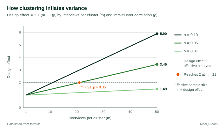
Two rules of thumb help explain where design effects come from. For clustering, with an average of m interviews per cluster and an intra-cluster correlation ρ:
deffcluster ≈ 1 + (m − 1) ρ
For variable weights, Kish (1992) showed that, when weights are unrelated to the survey variable, the loss of precision is approximately:
deffweights ≈ 1 + CV2
where CV is the coefficient of variation of the weights. Figure 1 shows how quickly clustering can erode precision. Even a modest intra-cluster correlation of 0.05, common for attitudes and behaviours that vary by area, doubles the variance when clusters contain about 21 interviews.
Design effects are useful for planning sample sizes and for explaining precision to clients, but they are summaries, not a method of analysis. They differ from one variable to another and from one estimate to another within the same survey, and those for subgroup estimates are usually smaller than those for the whole sample (Kish, 1965). For analysis, the variance should be estimated directly from the design.
The ultimate cluster approach
Most practical variance estimators rest on one simplification. Instead of modelling every stage of selection, they treat the primary sampling units (PSUs), the clusters selected at the first stage, as if they had been drawn with replacement within each stratum. All variation from later stages is then captured automatically in the variation between PSU totals. This is often called the ultimate cluster approach (Wolter, 2007). For an estimated total, the variance estimator becomes:
v(Ŷ) = Σh [nh ÷ (nh − 1)] Σi (ŷhi − ȳh)2
where nh is the number of PSUs in stratum h, ŷhi is the weighted total for PSU i, and ȳh is the mean of those totals in the stratum. The approximation is slightly conservative when the first-stage sampling fraction is small, which is usually the case.
This has a direct practical consequence. To estimate variance properly, the data file must identify the stratum and the PSU for each respondent, and each stratum must contain at least two PSUs. Survey files released for analysis typically include these variables, sometimes in masked form as "pseudo-strata" and "pseudo-PSUs" to protect confidentiality (Heeringa et al., 2010).
Method 1: Taylor series linearisation
Most estimates of interest are not simple totals. A mean is a ratio of two totals (the weighted sum of the variable divided by the sum of weights), and regression coefficients, correlations and odds ratios are more complex functions still. Taylor series linearisation approximates each such statistic by a linear function of estimated totals, then applies the variance formula for totals. For a ratio R̂ = Ŷ ÷ X̂:
v(R̂) ≈ (1 ÷ X̂2) [v(Ŷ) + R̂2 v(X̂) − 2R̂ cov(Ŷ, X̂)]
Woodruff (1971) showed how to carry this out conveniently by computing a "linearised variable" for each respondent and applying the total-variance formula to it. Binder (1983) extended the approach to any estimator defined by estimating equations, which covers linear, logistic and many other regression models. Linearisation is the default in most survey software, is fast, and needs only the strata, PSU and weight variables (Lumley, 2010).
Its limitations are that each new type of statistic needs its own derivation, and that it does not apply directly to non-smooth statistics such as medians and other percentiles. For these, specialised methods based on confidence intervals for the distribution function are used (Francisco & Fuller, 1991).
Method 2: replication methods
Replication methods take a different route. They form many subsamples, or reweighted versions of the full sample, recompute the estimate for each one, and use the spread of these replicate estimates to measure variance. The same procedure works for any statistic, which is their great advantage (Rust & Rao, 1996; Wolter, 2007). In practice, replication is implemented through replicate weights: extra weight columns in the data file, each defining one replicate.
Balanced repeated replication (BRR) is designed for surveys with exactly two PSUs per stratum. Each replicate keeps one PSU from every stratum, chosen according to a balanced pattern so that the replicates together reproduce the full-sample variance for linear statistics (McCarthy, 1969). The variance estimate is the average squared deviation of the R replicate estimates from the full-sample estimate:
vBRR(θ̂) = (1 ÷ R) Σr (θ̂r − θ̂)2
Fay's variant perturbs the weights rather than dropping half the sample, multiplying them by a factor such as 0.5 or 1.5 instead of 0 or 2. This avoids unstable replicates when estimates are based on small domains (Rust & Rao, 1996).
The jackknife drops one PSU at a time, reweights the remaining PSUs in its stratum, and recomputes the estimate. The stratified jackknife estimator is:
vJK(θ̂) = Σh [(nh − 1) ÷ nh] Σi (θ̂(hi) − θ̂)2
It works well for smooth statistics such as means, ratios and regression coefficients, but is known to be inconsistent for medians and other quantiles (Efron, 1979).
The bootstrap resamples PSUs with replacement within each stratum (Efron, 1979). Naive resampling gives biased variance estimates when strata contain few PSUs, so survey versions rescale the weights to correct for this. The rescaling bootstrap of Rao and Wu (1988), and the practical version that draws nh − 1 PSUs per stratum (Rao et al., 1992), are widely used by national statistical agencies, which release hundreds of bootstrap weights with their microdata. The bootstrap also handles quantiles well. Mashreghi et al. (2016) review the many bootstrap variants for finite population sampling.
Krewski and Rao (1981) showed that linearisation, the jackknife and BRR are asymptotically equivalent for smooth statistics in stratified samples, so in large surveys the choice is often driven by practicality rather than accuracy.
| Method | Works for | Needs in the data file | Main strengths | Main limitations |
|---|---|---|---|---|
| Linearisation | Smooth statistics | Strata, PSUs, weights | Fast; default in software | Separate derivation per statistic; not for quantiles |
| BRR / Fay | Most statistics | Replicate weights | General; hides design codes | Designed for two PSUs per stratum |
| Jackknife | Smooth statistics | Replicate weights or strata and PSUs | General and simple | Unreliable for quantiles |
| Bootstrap | Most statistics, including quantiles | Replicate weights or strata and PSUs | General; good for quantiles | Many replicates; Monte Carlo noise |
Weighting adjustments and imputation
Final survey weights are rarely just inverse selection probabilities. They are adjusted for nonresponse and then calibrated so that weighted totals match known population figures, such as age, sex and region distributions from a census (Deville & Särndal, 1992). Calibration has a real effect on variance: for variables strongly related to the calibration totals it can reduce variance substantially, while for unrelated variables the extra weight variation can increase it. Linearisation handles calibration through the residuals of a regression on the calibration variables (Särndal et al., 1992). With replication, each set of replicate weights should go through the same nonresponse and calibration steps as the full-sample weights, so that their effect is reflected in the spread of the replicates (Valliant et al., 2018). Analysts who build replicates from the base weights and then apply the final weights only to the full sample will misstate the variance.
Imputed values raise a similar problem. If missing answers are filled in and then treated as real data, standard errors are too small because the uncertainty of imputation is ignored. Rao and Shao (1992) proposed an adjusted jackknife for hot-deck imputation in which the imputed values are recomputed for each replicate. Multiple imputation is a widely used alternative.
A worked example
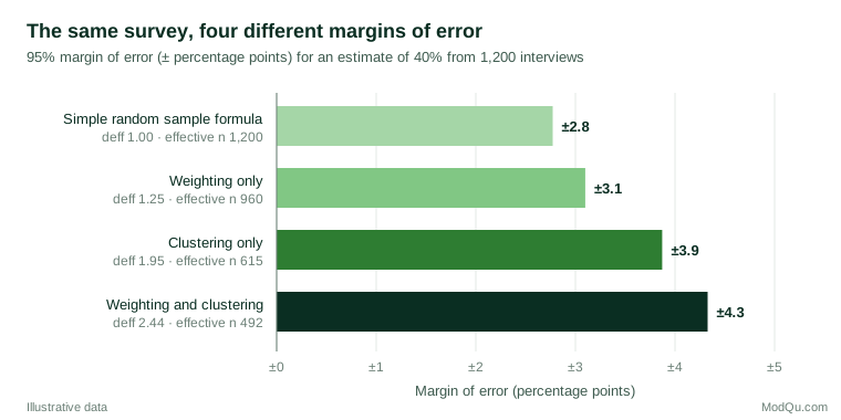
Suppose a hypothetical national brand-tracking survey interviews 1,200 adults. The design selects 60 neighbourhoods (PSUs) in six regional strata, with 20 interviews per neighbourhood, and the final weights have a coefficient of variation of 0.5. The survey estimates that 40% of adults are aware of a new product.
The simple random sampling formula gives a standard error of √(0.4 × 0.6 ÷ 1,200) = 1.41 percentage points, and a 95% margin of error of ±2.8 points. Now apply the design. With an intra-cluster correlation of 0.05 for brand awareness (an illustrative value), the clustering design effect is 1 + 19 × 0.05 = 1.95. The weighting design effect is 1 + 0.52 = 1.25. Multiplying the two, a common approximation, gives an overall design effect of about 2.44.
The design-based standard error is therefore 1.41 × √2.44 ≈ 2.21 points, and the 95% margin of error is about ±4.3 points. The effective sample size is 1,200 ÷ 2.44 ≈ 492. In practice the analyst would compute the standard error directly by linearisation or replicate weights, but the approximation shows why the answer differs so much from the naive one.
There is a second consequence. With 60 PSUs in six strata, the design provides only about 60 − 6 = 54 degrees of freedom for variance estimation, not 1,199. For overall estimates this makes little difference, but for small subgroups that fall in only a few PSUs, or for tests involving many parameters, it can matter a great deal (Heeringa et al., 2010).
Comparisons, changes and published tables
Business users rarely want a single estimate. They want to know whether awareness rose since the last wave, or whether satisfaction differs between two regions. The variance of a difference is the sum of the two variances minus twice their covariance, and in complex samples that covariance is often far from zero. Two subgroups drawn from the same clusters share cluster effects. Two waves of a tracking study that reuse the same neighbourhoods, or the same panel members, are positively correlated, which makes estimates of change more precise than a naive comparison would suggest. Treating the two estimates as independent therefore usually overstates the uncertainty of change in a panel and can hide real movements. The simplest safe approach is to compute the difference within one analysis that carries the full design for both groups or waves. With replicate weights, this is automatic: compute the difference in each replicate and take the spread of those differences (Wolter, 2007).
Agencies that publish thousands of table cells cannot print a standard error for each one. A common solution is the generalised variance function, a fitted curve that relates the relative variance of an estimate to its size. Readers can then approximate the standard error of any published figure from a short table of coefficients (Wolter, 2007). These functions are convenient, but they are averages over many variables and should not replace direct estimation when microdata are available.
Finally, the variance estimate itself is uncertain. With few PSUs, it rests on a small number of degrees of freedom, and t rather than normal critical values should be used for intervals (Lohr, 2021).
Tests and models with complex samples
Variance estimation affects more than confidence intervals. The standard Pearson chi-square test for a cross-tabulation assumes independent observations and, with clustered data, rejects true null hypotheses far too often. Rao and Scott (1981) developed corrections that divide the test statistic by an estimate of the average design effect, and these are now standard in survey software. For regression models, design-based standard errors from linearisation or replication should replace the model-based ones, and Wald tests should use degrees of freedom based on the number of PSUs (Lumley, 2010).
Practical guidance
- Use the design information you have been given. If a data file contains stratum, PSU and weight variables, or replicate weights, use them with survey procedures. Most statistical packages have them, and the documentation usually specifies the intended method (Statistics Canada, 2010).
- Do not treat the weight as a frequency count. Telling ordinary software that a respondent with a weight of 250 represents 250 independent observations produces wildly overconfident results.
- Analyse subgroups within the full design. Deleting cases outside a subgroup before analysis can remove whole PSUs or strata and distort the variance. Survey software provides domain (subpopulation) analysis for this purpose (Lohr, 2021).
- Report design effects or effective sample sizes alongside key results, so that readers understand the real precision.
- Plan sample sizes with design effects in mind. A target margin of ±3 points with an expected design effect of 2 needs about twice the sample size of a simple random sample.
- Watch for strata with a single PSU, which often arise after subsetting or nonresponse. They must be collapsed with similar strata or handled with a specific option; otherwise variance estimates fail or are understated.
- Choose replication for complex statistics. For medians, Gini coefficients or statistics computed by multistep procedures, bootstrap replicate weights are usually the simplest reliable option.
Common mistakes
- Ignoring the design entirely. A review of published secondary analyses of major survey data sets by West et al. (2016) found that many failed to account for the design features correctly, which typically leads to standard errors that are too small and findings that look stronger than they are.
- Using weights but not strata and PSUs. Weighted estimates are then correct, but their standard errors still ignore clustering.
- Recalculating weights without recalculating replicates. Any change to the weights, such as a new calibration, must be applied to every replicate as well.
- Assuming one design effect fits all variables. Design effects for demographic variables, attitudes and behaviours can differ widely within the same survey.
- Applying design-based variance formulas to nonprobability samples as if they had known selection probabilities. Variance estimates from opt-in panels depend on modelling assumptions and should be presented with caution.
Key takeaways
Complex survey designs change the precision of estimates, so standard errors must reflect stratification, clustering, weighting and calibration. Design effects summarise the impact and are valuable for planning, but analysis should estimate variance directly. Taylor series linearisation is fast and standard for smooth statistics. Replication methods, including BRR, the jackknife and the bootstrap, work for almost any statistic and allow agencies to release replicate weights instead of design codes. Whatever method is used, the data file must carry the design information, subgroup analyses should keep the full design, and reported margins of error should be honest about the real effective sample size.
References
Binder, D. A. (1983). On the variances of asymptotically normal estimators from complex surveys. International Statistical Review, 51(3), 279–292. https://doi.org/10.2307/1402588
Deville, J.-C., & Särndal, C.-E. (1992). Calibration estimators in survey sampling. Journal of the American Statistical Association, 87(418), 376–382. https://doi.org/10.1080/01621459.1992.10475217
Efron, B. (1979). Bootstrap methods: Another look at the jackknife. The Annals of Statistics, 7(1), 1–26. https://doi.org/10.1214/aos/1176344552
Francisco, C. A., & Fuller, W. A. (1991). Quantile estimation with a complex survey design. The Annals of Statistics, 19(1), 454–469. https://doi.org/10.1214/aos/1176347993
Heeringa, S. G., West, B. T., & Berglund, P. A. (2010). Applied survey data analysis. Chapman and Hall/CRC. https://doi.org/10.1201/9781420080674
Horvitz, D. G., & Thompson, D. J. (1952). A generalization of sampling without replacement from a finite universe. Journal of the American Statistical Association, 47(260), 663–685. https://doi.org/10.1080/01621459.1952.10483446
Kish, L. (1965). Survey sampling. Wiley.
Kish, L. (1992). Weighting for unequal Pi. Journal of Official Statistics, 8(2), 183–200.
Krewski, D., & Rao, J. N. K. (1981). Inference from stratified samples: Properties of the linearization, jackknife and balanced repeated replication methods. The Annals of Statistics, 9(5), 1010–1019. https://doi.org/10.1214/aos/1176345580
Lohr, S. L. (2021). Sampling: Design and analysis (3rd ed.). Chapman and Hall/CRC. https://doi.org/10.1201/9780429298899
Lumley, T. (2010). Complex surveys: A guide to analysis using R. Wiley. https://doi.org/10.1002/9780470580066
Mashreghi, Z., Haziza, D., & Léger, C. (2016). A survey of bootstrap methods in finite population sampling. Statistics Surveys, 10, 1–52. https://doi.org/10.1214/16-SS113
McCarthy, P. J. (1969). Pseudo-replication: Half samples. Review of the International Statistical Institute, 37(3), 239–264. https://doi.org/10.2307/1402116
Rao, J. N. K., & Scott, A. J. (1981). The analysis of categorical data from complex sample surveys: Chi-squared tests for goodness of fit and independence in two-way tables. Journal of the American Statistical Association, 76(374), 221–230. https://doi.org/10.1080/01621459.1981.10477633
Rao, J. N. K., & Shao, J. (1992). Jackknife variance estimation with survey data under hot deck imputation. Biometrika, 79(4), 811–822. https://doi.org/10.1093/biomet/79.4.811
Rao, J. N. K., & Wu, C. F. J. (1988). Resampling inference with complex survey data. Journal of the American Statistical Association, 83(401), 231–241. https://doi.org/10.1080/01621459.1988.10478591
Rao, J. N. K., Wu, C. F. J., & Yue, K. (1992). Some recent work on resampling methods for complex surveys. Survey Methodology, 18(2), 209–217.
Rust, K. F., & Rao, J. N. K. (1996). Variance estimation for complex surveys using replication techniques. Statistical Methods in Medical Research, 5(3), 283–310. https://doi.org/10.1177/096228029600500305
Särndal, C.-E., Swensson, B., & Wretman, J. (1992). Model assisted survey sampling. Springer. https://doi.org/10.1007/978-1-4612-4378-6
Statistics Canada. (2010). Survey methods and practices (Catalogue No. 12-587-X). https://www150.statcan.gc.ca/n1/en/catalogue/12-587-X
Valliant, R., Dever, J. A., & Kreuter, F. (2018). Practical tools for designing and weighting survey samples (2nd ed.). Springer. https://doi.org/10.1007/978-3-319-93632-1
West, B. T., Sakshaug, J. W., & Aurelien, G. A. S. (2016). How big of a problem is analytic error in secondary analyses of survey data? PLOS ONE, 11(6), Article e0158120. https://doi.org/10.1371/journal.pone.0158120
Wolter, K. M. (2007). Introduction to variance estimation (2nd ed.). Springer. https://doi.org/10.1007/978-0-387-35099-8
Woodruff, R. S. (1971). A simple method for approximating the variance of a complicated estimate. Journal of the American Statistical Association, 66(334), 411–414. https://doi.org/10.1080/01621459.1971.10482279