
Statistics · Survey statistics
Analysing Likert Scale Data: Ordinal or Interval?
Whether agree–disagree ratings can be averaged has been argued for seventy years. This article explains both positions, the evidence behind them, and a practical way to analyse and report Likert data.
Few survey questions are as familiar as the agreement item: "The checkout process was easy to use", answered on a scale from strongly disagree to strongly agree. Few questions also cause as much statistical argument. Some textbooks say these answers are ordinal and must never be averaged. Others say that means and t-tests are perfectly acceptable. Both camps cite respected authorities, and both are partly right. This article explains where the disagreement comes from, what the evidence shows, and how to choose an analysis that a business audience can trust.
What a Likert scale is
Rensis Likert introduced the method in 1932 as a way to measure attitudes. Respondents rated a series of statements on the same agreement format, and their answers were scored and summed across statements to give a single attitude score (Likert, 1932). Two terms are therefore worth separating:
- A Likert item is one statement with its ordered response options, usually five or seven.
- A Likert scale is the total or average of several items designed to measure the same construct, such as trust in a brand or satisfaction with service.
Much of the confusion in the literature comes from mixing the two (Carifio & Perla, 2007; Harpe, 2015). An individual item has only a handful of possible values. A scale built from ten items has dozens of possible values and behaves much more like a continuous measurement. Many survey questions that people call "Likert scales" are, strictly, single Likert-type items.
Where the debate comes from
The argument goes back to Stevens (1946), who classified measurements into four levels of measurement: nominal, ordinal, interval and ratio. On an ordinal scale, the categories have a meaningful order, but the distances between them are unknown. On an interval scale, equal differences in numbers represent equal differences in the property measured. Stevens argued that each level permits certain statistics: medians and percentiles for ordinal data, means and standard deviations only from the interval level upwards.
Agreement responses clearly have an order. Whether they have equal intervals is far less clear. Is the step from disagree to neutral the same size as the step from agree to strongly agree? Nothing in the questionnaire guarantees it. On a strict reading of Stevens, the codes 1 to 5 are labels in order, not quantities, and averaging them is not permitted.
Critics replied almost immediately. In a famous satirical note, Lord (1953) described a professor who computed means of football players' jersey numbers and concluded that "the numbers don't know where they came from". The point was that a statistical test asks a question about numbers; whether the answer means anything is a separate question about measurement. Gaito (1980) argued that tying the choice of statistical test to the level of measurement was a misconception. Townsend and Ashby (1984) answered that it was this criticism that was mistaken, because a statement such as "group A has a higher mean than group B" can change direction when the scale is transformed in an order-preserving way. Michell (1986) showed that the participants were working from different theories of what measurement is, and Velleman and Wilkinson (1993) concluded that Stevens's typology is a poor guide for choosing statistical methods in practice.
The debate has never been settled, partly because each side is answering a different question. Kampen and Swyngedouw (2000), revisiting this "ordinal controversy", stressed that the real issue is what an analyst is willing to assume about the distances between categories.
The case for treating Likert data as ordinal
Jamieson (2004) set out the ordinal position clearly for applied researchers. The response categories are ranks, intervals between them cannot be presumed equal, and the appropriate summaries are the median, the mode and the frequency distribution. Group comparisons should use non-parametric tests based on ranks, such as the Mann–Whitney test (Mann & Whitney, 1947), or methods designed for ordinal outcomes.
This position has three strong practical arguments behind it.
- The mean can hide important differences. Two products with the same mean score can have very different response patterns, as the example below shows.
- Real items are often skewed or bunched at the ends. Ceiling effects, where most respondents choose the top category, make means and standard deviations hard to interpret.
- Metric analyses can give wrong answers. Liddell and Kruschke (2018), using simulations and reanalyses of published data, showed that treating ordinal responses as metric can produce false alarms, missed differences and even reversed conclusions about which group scores higher, particularly when the groups differ in the spread of their underlying attitudes.
The case for treating Likert data as interval
Norman (2010) set out the opposite position. Parametric methods such as the t-test, analysis of variance and linear regression are robust: they give accurate answers even when their assumptions are violated, including when data are skewed, samples are small and variances are unequal. In his view, researchers can use them on Likert data "with no fear" of reaching the wrong conclusion, a phrase that has been widely quoted ever since.
Several lines of evidence support the interval approach, at least for some types of data:
- Summed scales behave like continuous data. Carifio and Perla (2007) argued that criticisms aimed at single items had been wrongly applied to multi-item scales, which were what Likert designed and which typically have many possible values and roughly symmetric distributions.
- Large samples protect the mean. Lumley et al. (2002) showed that t-tests and linear regression remain valid in large samples whatever the shape of the distribution, because the sampling distribution of the mean becomes approximately normal.
- More response categories help. In a simulation study, Wu and Leung (2017) found that Likert data approximated interval data more closely as the number of scale points increased.
- Five or more categories are often enough for modelling. Rhemtulla et al. (2012) compared estimation methods in confirmatory factor analysis and found that, with five or more response categories, robust continuous methods performed about as well as methods designed for categorical data. With fewer categories, the categorical methods were better.
A worked example: the same mean, different stories
Suppose a hypothetical customer survey asks 500 users of each of two products whether they agree that "the product meets my needs". Figure 1 shows the responses.
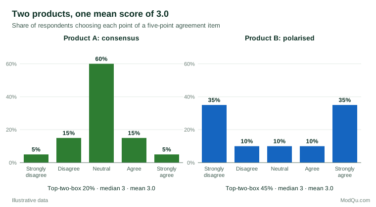
Both products have a mean of 3.0 and a median of 3. A report that showed only the average would describe them as identical. Yet Product A is met with mild indifference, while Product B has a large group of enthusiasts and an equally large group of dissatisfied users. The commercial implications are completely different: Product B may need fixing for one segment and protecting for another.
| Summary | Product A | Product B |
|---|---|---|
| Mean (1–5) | 3.0 | 3.0 |
| Standard deviation | 0.84 | 1.73 |
| Median | 3 | 3 |
| Top-two-box (agree or strongly agree) | 20% | 45% |
| Bottom-two-box (disagree or strongly disagree) | 20% | 45% |
The example makes a point that is often missed in the debate: the median does not solve the problem either. What reveals the difference is the full distribution, or summaries of it such as top-two-box and bottom-two-box percentages, or the standard deviation. The lesson is not that means are forbidden, but that no single number can describe an ordinal item.
A latent-variable view
A useful way to reconcile the two positions is to imagine that each response reflects a continuous underlying attitude, which the respondent maps onto the nearest answer category. The categories are separated by thresholds on this latent scale. If the thresholds were equally spaced and the latent attitude were roughly normal, the codes 1 to 5 would behave much like interval data. If the thresholds are unequally spaced, they will not.
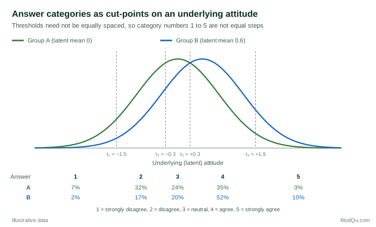
In Figure 2, the neutral band is narrow and the agree band is wide, which is common when people are reluctant to choose the extreme category. A shift of 0.6 standard deviations in the latent attitude moves the mean score from 2.96 to 3.51 here, but the same latent shift would produce a different change in the mean score if the two groups started from a different part of the scale. This is the mechanism behind the distortions described by Liddell and Kruschke (2018). It is also the basis of the models designed for ordinal data.
Methods designed for ordinal data
Analysts who want to respect the ordinal nature of the data are no longer restricted to simple rank tests. Ordinal regression, especially the proportional odds model introduced by McCullagh (1980), estimates the thresholds directly from the data and models how explanatory variables shift the latent attitude. It handles several predictors, interactions and covariates, just like linear regression, and reports effects as odds ratios or as predicted probabilities of each response category (Agresti, 2010). Bayesian versions are also available and are well suited to surveys with many items or groups (Bürkner & Vuorre, 2019).
For simpler comparisons, rank-based tests such as the Mann–Whitney test compare whether responses in one group tend to be higher than in another. They answer a slightly different question from a t-test, about the probability that a randomly chosen respondent in one group gives a higher rating than one in the other, which is often a natural question for business audiences.
A practical decision guide
The evidence supports a pragmatic middle path rather than a blanket rule. Harpe (2015) reached a similar position after reviewing the literature, and Sullivan and Artino (2013) also advise describing single items with frequencies while accepting that parametric tests are generally robust.
Single items
- Always report the full distribution, or at least top-box and bottom-box percentages, alongside any average.
- Means are acceptable as a supplementary summary for items with five or more categories and reasonably large samples, provided they are not the only figure shown and the distribution is not heavily skewed or polarised.
- Use ordinal regression or rank-based tests when the item is a key outcome, when the distribution is bunched at one end, or when the groups compared appear to differ in spread. These methods avoid the distortions that metric models can introduce.
Multi-item scales
- Means, t-tests, analysis of variance and linear regression are generally appropriate for well-constructed scales that sum or average several items. Check the scale's reliability and, where relevant, its factor structure first.
- Look at the distribution of the scale score. Strong ceiling effects still call for caution.
Design choices
The analysis is easier when the questionnaire is designed with it in mind. Labelled categories with balanced wording and a clear midpoint help respondents use the scale consistently. Revilla et al. (2014) compared agree–disagree scales with different numbers of categories and found that five categories gave better measurement quality than seven or eleven, so adding categories is not automatically an improvement for agreement items. When a near-continuous measure is needed, a multi-item scale is usually a better investment than a longer single item.
Reporting Likert results
Good reporting matters as much as the choice of test, because most readers of a survey report will never see the analysis behind it. A compact, honest presentation of a key agreement item usually includes four elements:
- A stacked or diverging bar chart showing the share of respondents in every category, with the neutral group visible rather than hidden. Diverging charts, which place disagreement to the left of a central line and agreement to the right, make comparisons across many items or segments easy to read.
- Top-box and bottom-box percentages with their margins of error. "45% agree" is easier to act on than "a mean of 3.0", and the percentage has a direct interpretation as a share of customers.
- The unweighted base for each group, so that readers can judge how much weight to place on small segments.
- A note on the method used for any significance test, for example "differences tested with ordinal logistic regression" or "two-sample t-test on the scale score".
When a mean is shown, label the scale so that readers know what 1 and 5 stand for, and avoid decimal precision that the data cannot support. A change from 3.42 to 3.47 is almost never meaningful for a single item, however large the sample.
Tracking studies need special care. If the wording, the number of categories or the order of the response options changes between waves, the response distribution can shift even when attitudes have not. Keep the item identical across waves, or run old and new versions side by side for one wave before switching, so that a genuine change can be separated from an artefact of the questionnaire.
Common mistakes
- Reporting only a mean for a single item. As Figure 1 shows, averages can conceal polarisation and other patterns that matter commercially.
- Treating the median as the solution. With only five categories, medians are coarse and often identical across groups that differ substantially.
- Applying the ordinal rule to multi-item scales. Averaged scales are not the same as single items and can usually be analysed with standard methods (Carifio & Perla, 2007).
- Comparing means across groups with very different spreads. This is where metric analysis is most likely to mislead (Liddell & Kruschke, 2018).
- Combining items with different response formats without checking. Summing a five-point item with a ten-point item gives the second more influence.
- Assuming the numbers carry meaning. A mean of 3.4 on a five-point item does not tell a manager how many customers are satisfied. Percentages usually communicate better.
Key takeaways
Likert items are ordinal by construction, while multi-item Likert scales often behave close enough to interval data for standard methods to work well. The real risk is not computing a mean but relying on one number when the distribution matters, or comparing means between groups that use the scale differently. For single items, show the distribution and consider ordinal regression for key outcomes; for summed scales, standard parametric methods are usually sound. Above all, choose the analysis by the question being asked, and present results in a form that decision-makers can interpret correctly.
References
Agresti, A. (2010). Analysis of ordinal categorical data (2nd ed.). Wiley. https://doi.org/10.1002/9780470594001
Bürkner, P.-C., & Vuorre, M. (2019). Ordinal regression models in psychology: A tutorial. Advances in Methods and Practices in Psychological Science, 2(1), 77–101. https://doi.org/10.1177/2515245918823199
Carifio, J., & Perla, R. J. (2007). Ten common misunderstandings, misconceptions, persistent myths and urban legends about Likert scales and Likert response formats and their antidotes. Journal of Social Sciences, 3(3), 106–116. https://doi.org/10.3844/jssp.2007.106.116
Gaito, J. (1980). Measurement scales and statistics: Resurgence of an old misconception. Psychological Bulletin, 87(3), 564–567. https://doi.org/10.1037/0033-2909.87.3.564
Harpe, S. E. (2015). How to analyze Likert and other rating scale data. Currents in Pharmacy Teaching and Learning, 7(6), 836–850. https://doi.org/10.1016/j.cptl.2015.08.001
Jamieson, S. (2004). Likert scales: How to (ab)use them. Medical Education, 38(12), 1217–1218. https://doi.org/10.1111/j.1365-2929.2004.02012.x
Kampen, J., & Swyngedouw, M. (2000). The ordinal controversy revisited. Quality and Quantity, 34(1), 87–102. https://doi.org/10.1023/A:1004785723554
Liddell, T. M., & Kruschke, J. K. (2018). Analyzing ordinal data with metric models: What could possibly go wrong? Journal of Experimental Social Psychology, 79, 328–348. https://doi.org/10.1016/j.jesp.2018.08.009
Likert, R. (1932). A technique for the measurement of attitudes. Archives of Psychology, 22(140), 1–55.
Lord, F. M. (1953). On the statistical treatment of football numbers. American Psychologist, 8(12), 750–751. https://doi.org/10.1037/h0063675
Lumley, T., Diehr, P., Emerson, S., & Chen, L. (2002). The importance of the normality assumption in large public health data sets. Annual Review of Public Health, 23(1), 151–169. https://doi.org/10.1146/annurev.publhealth.23.100901.140546
Mann, H. B., & Whitney, D. R. (1947). On a test of whether one of two random variables is stochastically larger than the other. The Annals of Mathematical Statistics, 18(1), 50–60. https://doi.org/10.1214/aoms/1177730491
McCullagh, P. (1980). Regression models for ordinal data. Journal of the Royal Statistical Society Series B: Statistical Methodology, 42(2), 109–127. https://doi.org/10.1111/j.2517-6161.1980.tb01109.x
Michell, J. (1986). Measurement scales and statistics: A clash of paradigms. Psychological Bulletin, 100(3), 398–407. https://doi.org/10.1037/0033-2909.100.3.398
Norman, G. (2010). Likert scales, levels of measurement and the "laws" of statistics. Advances in Health Sciences Education, 15(5), 625–632. https://doi.org/10.1007/s10459-010-9222-y
Revilla, M. A., Saris, W. E., & Krosnick, J. A. (2014). Choosing the number of categories in agree–disagree scales. Sociological Methods & Research, 43(1), 73–97. https://doi.org/10.1177/0049124113509605
Rhemtulla, M., Brosseau-Liard, P. É., & Savalei, V. (2012). When can categorical variables be treated as continuous? A comparison of robust continuous and categorical SEM estimation methods under suboptimal conditions. Psychological Methods, 17(3), 354–373. https://doi.org/10.1037/a0029315
Stevens, S. S. (1946). On the theory of scales of measurement. Science, 103(2684), 677–680. https://doi.org/10.1126/science.103.2684.677
Sullivan, G. M., & Artino, A. R., Jr. (2013). Analyzing and interpreting data from Likert-type scales. Journal of Graduate Medical Education, 5(4), 541–542. https://doi.org/10.4300/JGME-5-4-18
Townsend, J. T., & Ashby, F. G. (1984). Measurement scales and statistics: The misconception misconceived. Psychological Bulletin, 96(2), 394–401. https://doi.org/10.1037/0033-2909.96.2.394
Velleman, P. F., & Wilkinson, L. (1993). Nominal, ordinal, interval, and ratio typologies are misleading. The American Statistician, 47(1), 65–72. https://doi.org/10.1080/00031305.1993.10475938
Wu, H., & Leung, S.-O. (2017). Can Likert scales be treated as interval scales? A simulation study. Journal of Social Service Research, 43(4), 527–532. https://doi.org/10.1080/01488376.2017.1329775