
Statistics · Survey statistics
Statistical Analysis of Weighted Survey Data
How survey weights, strata and clusters change standard errors, how design effects and replication methods measure the change, and how to analyse subgroups and fit models correctly.
Most published survey results are weighted. A separate ModQu article on weighted means and weighted percentages explains how weights correct a sample that does not match its population. This article goes one step further: once the weights are in place, how should the data be analysed? The short answer is that weighted point estimates are only half the job. Standard errors, confidence intervals, significance tests and regression output must also reflect the weights and the way the sample was drawn, or they will usually look more precise than they really are (Lohr, 2021; Heeringa et al., 2010).
What makes survey data "complex"
Textbook formulas assume a simple random sample: every member of the population had the same chance of selection and respondents were chosen independently. Real surveys rarely meet that standard. Three design features matter most.
- Weights. Each respondent carries a weight, starting from the inverse of their selection probability (Horvitz & Thompson, 1952) and then adjusted for nonresponse and to match known population totals through post-stratification, raking or calibration (Deville & Särndal, 1992; Kalton & Flores-Cervantes, 2003).
- Strata. The population is often divided into groups, such as regions or customer tiers, and sampled separately within each. Stratification usually improves precision.
- Clusters. To save cost, surveys often sample groups first, such as stores, schools or postal areas, and then people within them. People in the same cluster tend to resemble one another, so clustering usually reduces precision.
A dataset with these features is called a complex sample. Analysing it as if it were a simple random sample ignores all three.
The design effect
Kish (1965) summarised the combined impact of a design in a single number, the design effect, or deff: the variance of an estimate under the actual design divided by its variance under a simple random sample of the same size.
deff = Vardesign(θ̂) ÷ VarSRS(θ̂)
A deff of 2 means the survey has twice the variance a simple random sample would have, so confidence intervals are about 1.41 times as wide (the square root of 2). The effective sample size is the number of interviews divided by the design effect: the size of a simple random sample that would give the same precision.
The weighting component
Unequal weights alone inflate variance. Kish (1992) gave a widely used approximation for this part of the design effect, based only on the weights:
deffw = n Σ wi² ÷ (Σ wi)² = 1 + CVw²
where CVw is the coefficient of variation of the weights. Weights with a coefficient of variation of 0.6, which is common after heavy post-stratification, give deffw = 1.36. This formula is a planning and reporting tool. It assumes the outcome is unrelated to the weights, and it ignores clustering and stratification, so it is not a substitute for design-based variance estimation.
The clustering component
For clusters of average size m and an intraclass correlation ρ, which measures how similar people in the same cluster are, Kish (1965) gave the approximation:
deffc = 1 + (m − 1)ρ
Even a small ρ matters when clusters are large. With 20 interviews per cluster and ρ = 0.02, the clustering deff is 1.38.
A worked example
Consider a hypothetical customer survey of 2,000 people interviewed in 100 stores, 20 per store, and weighted to match the customer base by age, region and spending tier. The weighted share of satisfied customers is 42%.
| Method | Design effect | 95% margin of error | Effective n |
|---|---|---|---|
| Simple random sampling formula | 1.00 | ±2.2 points | 2,000 |
| Weights only (Kish approximation) | 1.36 | ±2.5 points | 1,471 |
| Weights and clustering | 1.88 | ±3.0 points | 1,066 |
The naive analysis understates the margin of error by about a quarter. A difference of 2.5 points between this survey and last year's might look significant under the naive formula and not under the correct one.
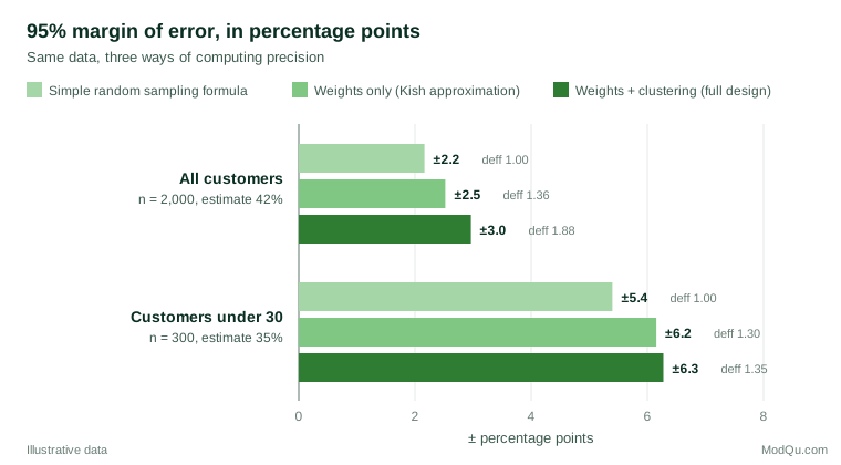
The subgroup of 300 customers under 30 behaves differently. Its weights vary slightly less, and with only about three respondents per store the clustering effect almost disappears. Design effects are specific to each estimate and each subgroup, which is why analysts should compute them rather than apply one survey-wide figure (Kish, 1965; Lohr, 2021).
How design-based variance is estimated
Modern software does not rely on the approximations above. It estimates variance directly from the design information stored in the dataset: the weight, the stratum and the primary sampling unit (cluster) of each respondent. Two families of methods dominate (Wolter, 2007).
Taylor series linearisation approximates a nonlinear statistic, such as a ratio or a regression coefficient, by a linear one and then applies the variance formula for stratified cluster samples to the linearised values (Fuller, 2009; Särndal et al., 1992). It is fast and is the default in most packages.
Replication methods repeatedly recompute the estimate on subsamples of clusters and measure how much it varies. The jackknife, balanced repeated replication and the bootstrap are the main variants (Wolter, 2007). Data producers often release a set of replicate weights instead of stratum and cluster codes, which protects respondents' confidentiality while still allowing correct variance estimation. Replication also captures the variance added by nonresponse adjustment and calibration when those steps are repeated for each replicate (Valliant et al., 2018).
Both approaches agree closely in large samples. The important choice is to use one of them rather than neither.
Analysing subgroups
Business users almost always want results by region, segment or demographic group. Survey statisticians call these subgroups domains, and they require care (Heeringa et al., 2010; Lumley, 2010).
- Do not delete the other cases. Filtering the dataset to one subgroup before analysis can remove whole strata or clusters, and software then computes variance as though the subgroup's sample size had been fixed in advance. The correct approach keeps the full design and declares the subgroup as a domain, for example with a subpopulation option.
- Report the unweighted base. A subgroup with 60 interviews but a large weighted total is still a 60-interview estimate. Many organisations set a minimum unweighted base for publication.
- Check the effective sample size. Small subgroups often contain a few respondents with very large weights. The Kish approximation, applied within the subgroup, flags these cases quickly.
- Compare subgroups with a design-based test. The difference between two domain estimates has its own standard error, which accounts for the fact that both come from the same sample.
Tests and models
Standard chi-square tests on weighted cross-tabulations are too liberal under complex designs, because the test statistic no longer follows its nominal distribution. Rao and Scott (1981, 1984) developed corrections that rescale the statistic using estimated design effects, and these Rao–Scott tests are now the standard for weighted contingency tables.
For regression, two questions arise. The first is variance: standard errors should always reflect clustering and stratification. The second is whether to use the weights for the coefficients themselves. For descriptive population quantities, such as the average satisfaction of all customers, weights are essential. For models that aim to describe a causal or structural relationship, the case is less clear-cut. Solon et al. (2015) show that weighting can correct for endogenous sampling and some forms of heterogeneity, but can also needlessly reduce precision, and they recommend comparing weighted and unweighted estimates as a diagnostic. A large difference signals that the model is misspecified or that effects vary across groups.
Software
All major statistical packages now support complex samples. In R, the survey package defines a design object once and then provides weighted means, totals, quantiles, domain estimates, Rao–Scott tests and generalised linear models (Lumley, 2010). Stata's svy prefix, SAS's SURVEY procedures and the complex samples module in SPSS offer similar functions (Heeringa et al., 2010). The common thread is that the analyst declares the weight, strata and clusters, or the replicate weights, before any analysis.
A frequent and costly error is to supply survey weights to ordinary procedures as "frequency weights". The software then treats the weighted total as the number of observations, which can turn 2,000 interviews into an apparent sample of hundreds of thousands and produce absurdly small standard errors. Weights rescaled to sum to the sample size avoid that extreme but still ignore the design.
Common mistakes
- Using weights for estimates but not for standard errors. The point estimate is right; the margin of error and every significance test are wrong.
- Ignoring clustering. When interviews are grouped by store, area or interviewer, the design effect from clustering can exceed the effect of the weights.
- Trimming or recalibrating weights without re-estimating variance. Any change to the weights changes the design effect (Kalton & Flores-Cervantes, 2003).
- Applying one design effect to every estimate. Design effects differ by variable and by subgroup, as the worked example shows.
- Omitting documentation. Analysts need the weight, strata and cluster variables, or replicate weights, and a description of how weights were built. Official statistical agencies provide this as standard (Statistics Canada, 2010).
Key takeaways
Weighted survey data needs weighted estimates and design-based measures of precision. The design effect summarises how much weights, strata and clusters change variance, and the effective sample size translates it into a figure decision-makers understand. Use linearisation or replicate weights through survey-aware software, treat subgroups as domains rather than separate datasets, use Rao–Scott tests for weighted tables, and report the unweighted base alongside every weighted result.
References
Deville, J.-C., & Särndal, C.-E. (1992). Calibration estimators in survey sampling. Journal of the American Statistical Association, 87(418), 376–382. https://doi.org/10.1080/01621459.1992.10475217
Fuller, W. A. (2009). Sampling statistics. Wiley. https://doi.org/10.1002/9780470523551
Heeringa, S. G., West, B. T., & Berglund, P. A. (2010). Applied survey data analysis. Chapman and Hall/CRC. https://doi.org/10.1201/9781420080674
Horvitz, D. G., & Thompson, D. J. (1952). A generalization of sampling without replacement from a finite universe. Journal of the American Statistical Association, 47(260), 663–685. https://doi.org/10.1080/01621459.1952.10483446
Kalton, G., & Flores-Cervantes, I. (2003). Weighting methods. Journal of Official Statistics, 19(2), 81–98.
Kish, L. (1965). Survey sampling. Wiley.
Kish, L. (1992). Weighting for unequal Pi. Journal of Official Statistics, 8(2), 183–200.
Lohr, S. L. (2021). Sampling: Design and analysis (3rd ed.). Chapman and Hall/CRC. https://doi.org/10.1201/9780429298899
Lumley, T. (2010). Complex surveys: A guide to analysis using R. Wiley. https://doi.org/10.1002/9780470580066
Rao, J. N. K., & Scott, A. J. (1981). The analysis of categorical data from complex sample surveys: Chi-squared tests for goodness of fit and independence in two-way tables. Journal of the American Statistical Association, 76(374), 221–230. https://doi.org/10.1080/01621459.1981.10477633
Rao, J. N. K., & Scott, A. J. (1984). On chi-squared tests for multiway contingency tables with cell proportions estimated from survey data. The Annals of Statistics, 12(1), 46–60. https://doi.org/10.1214/aos/1176346391
Särndal, C.-E., Swensson, B., & Wretman, J. (1992). Model assisted survey sampling. Springer. https://doi.org/10.1007/978-1-4612-4378-6
Solon, G., Haider, S. J., & Wooldridge, J. M. (2015). What are we weighting for? Journal of Human Resources, 50(2), 301–316. https://doi.org/10.3368/jhr.50.2.301
Statistics Canada. (2010). Survey methods and practices (Catalogue No. 12-587-X). https://www150.statcan.gc.ca/n1/en/catalogue/12-587-X
Valliant, R., Dever, J. A., & Kreuter, F. (2018). Practical tools for designing and weighting survey samples (2nd ed.). Springer. https://doi.org/10.1007/978-3-319-93632-1
Wolter, K. M. (2007). Introduction to variance estimation (2nd ed.). Springer. https://doi.org/10.1007/978-0-387-35099-8