
Statistics · Tests and models
Time Series Analysis and Forecasting
How to describe, model and forecast data collected over time, from trend and seasonality to exponential smoothing, ARIMA, forecast accuracy and honest prediction intervals for business planning.
Sales by month, website visits by day, brand awareness by survey wave and call-centre volumes by hour are all time series: measurements of the same quantity taken in order, usually at regular intervals. Businesses analyse them to understand what has happened and, above all, to forecast what will happen next. Staffing, stock, budgets and targets all depend on such forecasts.
Time series need their own methods because the observations are not independent. This month's sales are related to last month's, and to the same month last year. That dependence breaks the assumptions of ordinary regression, but it is also what makes forecasting possible: if the past carries information about the future, a model can extract it (Box & Jenkins, 1970; Shumway & Stoffer, 2017).
The building blocks: trend, seasonality and noise
Most business series can be described as a combination of a few components:
- Trend: the long-run direction, such as steady growth in enquiries as a brand becomes better known.
- Seasonality: a pattern that repeats over a fixed period, such as higher retail sales before Christmas, more travel bookings in January or weekly cycles in web traffic.
- Cycles: rises and falls of irregular length, often linked to the business cycle.
- Remainder: irregular variation that the other components do not explain.
In an additive decomposition the components add up, so seasonal swings are roughly constant in size. In a multiplicative decomposition they multiply, so swings grow with the level of the series; taking logarithms turns a multiplicative series into an additive one. A widely used procedure is STL, which estimates the trend and the seasonal pattern with locally weighted smoothing and lets the seasonal shape change slowly over time (Cleveland et al., 1990).
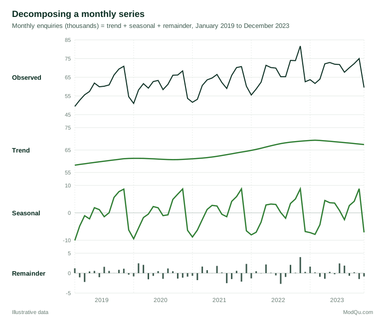
Decomposition is useful in its own right. A seasonally adjusted series (observed minus seasonal) shows whether a change from one month to the next is unusual or simply the time of year. Comparing November with October tells a manager little if November is always strong; comparing the adjusted figures does.
Autocorrelation and stationarity
The key descriptive tool for a time series is the autocorrelation function (ACF): the correlation between the series and itself shifted by one, two, three or more periods. A monthly series with strong seasonality shows a spike at lag 12. A series with a trend shows autocorrelations that decline only slowly.
Many models assume the series is stationary, meaning that its mean, variance and autocorrelation structure do not change over time. Trending or seasonal series are not stationary, but they can often be made so by differencing: modelling the change from one period to the next, or from the same month last year, rather than the level itself. Formal unit root tests, such as the Dickey–Fuller test, help decide whether differencing is needed (Dickey & Fuller, 1979).
Ignoring non-stationarity can be costly. Granger and Newbold (1974) showed that regressing one trending random series on another, completely unrelated one routinely produces high R² values and "significant" coefficients. Two business metrics that both grow over time will appear related even when neither influences the other. Analysing changes rather than levels, or using models designed for trending data, guards against such spurious regressions.
Forecasting methods
Simple benchmarks
Every forecasting exercise should start with simple benchmarks. The naive forecast says next period will equal this period. The seasonal naive forecast says next January will equal last January. The mean forecast uses the historical average. These methods are surprisingly hard to beat for some series, and a sophisticated model that cannot outperform them adds nothing (Hyndman & Athanasopoulos, 2021).
Exponential smoothing
Exponential smoothing produces forecasts from weighted averages of past observations, with weights that decline the further back they go. It was developed in the 1950s for inventory and sales planning, and Gardner (1985) reviews its early development. Simple exponential smoothing updates a single level:
ℓt = α yt + (1 − α) ℓt−1
where α, between 0 and 1, controls how quickly the level reacts to new data. Holt's method, first circulated in 1957 and later reprinted, adds a trend component (Holt, 2004), and Winters (1960) added seasonality, giving the Holt–Winters method that is still a workhorse of sales forecasting. Hyndman et al. (2002) placed these methods in a state space framework, known as ETS (error, trend, seasonal), which provides proper likelihoods, automatic model selection and prediction intervals.
ARIMA models
The second major family is ARIMA (autoregressive integrated moving average), popularised by Box and Jenkins (1970). An ARIMA model combines three ideas: autoregression, in which the current value depends on its own past values; integration, meaning that the series is differenced to make it stationary; and moving average terms, in which the current value depends on past forecast errors. Seasonal ARIMA models add the same terms at the seasonal lag. Box and Jenkins proposed an iterative cycle of identifying a model from the ACF, estimating it and checking its residuals. Today automatic algorithms search over candidate models using information criteria (Hyndman & Khandakar, 2008).
ETS and ARIMA overlap but are not identical. Exponential smoothing describes trend and seasonality directly, while ARIMA describes autocorrelation. In practice, analysts often fit both and compare their accuracy on held-out data.
Adding explanatory variables
Forecasts can also use outside information: prices, promotions, holidays, weather or advertising spend. Dynamic regression combines a regression on such predictors with ARIMA errors to capture the autocorrelation that remains. The catch is that future values of the predictors must themselves be known or forecast. A planned price change is known in advance, whereas next month's temperature is not. Calendar effects, such as the number of trading days in a month or the moving date of Easter, are cheap and dependable predictors for many monthly business series.
A worked example
Consider an illustrative series of monthly customer enquiries, in thousands, from January 2019 to December 2023 (Figure 1). We fit an additive Holt–Winters model (ETS with additive error, trend and seasonality) to these five years and forecast each month of 2024. We then compare the forecasts with what actually happened, a check known as holdout or out-of-sample evaluation.
The fitted level smoothing parameter is α ≈ 0.39, so the level adapts moderately to new data, while the seasonal pattern is estimated as almost fixed. Figure 2 shows the result. The forecast follows the seasonal shape, and the actual 2024 values fall inside the 80% prediction interval in 11 of the 12 months and inside the 95% interval in all of them. The forecast total for the year was 814 thousand against an actual 801 thousand, an error of under 2%.
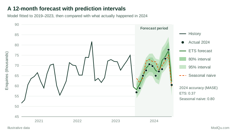
The seasonal naive benchmark, which simply repeats 2023, is less accurate. Its mean absolute percentage error over 2024 is 4.4%, against 2.0% for the exponential smoothing model.
Measuring forecast accuracy
Accuracy should always be judged on data the model has not seen. In-sample fit flatters complex models, which can mistake noise for pattern. A single holdout period is a start; rolling-origin evaluation, in which the model is refitted and forecasts are made repeatedly from successive starting points, gives a more reliable picture (Tashman, 2000).
Common accuracy measures each have strengths and weaknesses:
| Measure | What it shows | Watch out for |
|---|---|---|
| MAE (mean absolute error) | Typical error in the original units | Cannot compare series of different scale |
| RMSE (root mean squared error) | Like MAE but penalises large errors more | Sensitive to a few big misses |
| MAPE (mean absolute percentage error) | Error as a percentage, easy to explain | Undefined or explosive when actual values are near zero; treats over- and under-forecasts unevenly |
| MASE (mean absolute scaled error) | Error relative to a naive benchmark | Less familiar to business audiences |
Hyndman and Koehler (2006) proposed MASE, which divides the forecast error by the in-sample error of a naive method. A value below 1 means the forecast beats the benchmark. In the worked example, the exponential smoothing model has a MASE of 0.37 and the seasonal naive forecast 0.80, both scaled by the seasonal naive method's in-sample error.
Residual checks matter too. If the one-step forecast errors are still autocorrelated, the model has left usable information on the table. The Ljung–Box test checks a group of residual autocorrelations at once (Ljung & Box, 1978).
Prediction intervals and uncertainty
A point forecast alone invites false confidence. A prediction interval gives a range within which the future value is expected to fall with a stated probability, and it should widen as the forecast horizon lengthens. Chatfield (1993) noted that computed intervals tend to be too narrow, partly because they ignore uncertainty about which model is correct and assume the future will behave like the past. Good probabilistic forecasts should be both calibrated, so that 80% intervals contain the outcome about 80% of the time, and sharp, meaning as narrow as calibration allows (Gneiting et al., 2007). Tracking the coverage of past intervals is a simple and revealing check.
Combining forecasts and lessons from competitions
Averaging forecasts from different methods is one of the most reliable ways to improve accuracy. Clemen (1989) reviewed a large body of evidence showing that combining forecasts usually improves accuracy and that simple averages often perform as well as elaborate weighting schemes. Large forecasting competitions point the same way. In the M4 competition, with 100,000 series, most of the best-performing entries were combinations of methods or hybrids of statistical and machine learning approaches, while pure machine learning methods generally did poorly (Makridakis et al., 2020).
Practical guidance for survey and business data
- Separate sampling noise from real change in tracking studies. Each wave of a brand or satisfaction tracker carries sampling error. A three-point dip between waves of 300 respondents may be noise. Moving averages, smoothing or state space models help distinguish signal from noise.
- Watch for breaks. Changes to questionnaire wording, survey mode, sampling or weighting can shift a series overnight. Record them, and model them as level shifts rather than treating them as genuine change.
- Estimate the effect of interventions carefully. To judge whether a campaign moved sales, forecast what would have happened without it and compare. Brodersen et al. (2015) describe a Bayesian structural time-series approach to exactly this problem.
- Use judgement carefully. Managers often adjust statistical forecasts. In a study of supply-chain companies, Fildes et al. (2009) found that large adjustments tended to improve accuracy, whereas small adjustments did little good, and upward adjustments were much less likely to help than downward ones, consistent with optimism.
- Choose the horizon and level to match the decision. Daily staffing forecasts and annual budget forecasts call for different data, models and accuracy standards.
Common mistakes
- Judging models on in-sample fit rather than on genuinely held-out data.
- Regressing one trending series on another and reading the correlation as a relationship.
- Reporting a single number without an interval, or with intervals that are never checked against outcomes.
- Using MAPE for series with values near zero, such as intermittent demand.
- Extrapolating a trend indefinitely. Growth rates rarely persist, and trend forecasts for long horizons should be damped or treated with caution.
- Skipping the benchmark. If a model cannot beat the seasonal naive forecast, it should not be used.
Key takeaways
Time series analysis starts with understanding a series' trend, seasonality and autocorrelation. Exponential smoothing and ARIMA provide reliable, well-understood forecasting tools, and simple benchmarks keep them honest. Evaluate forecasts on held-out data with scale-free measures such as MASE, report prediction intervals and check their coverage, and consider combining methods. For survey trackers, remember that every wave carries sampling error and that methodological changes can masquerade as real movement.
References
Box, G. E. P., & Jenkins, G. M. (1970). Time series analysis: Forecasting and control. Holden-Day.
Brodersen, K. H., Gallusser, F., Koehler, J., Rémy, N., & Scott, S. L. (2015). Inferring causal impact using Bayesian structural time-series models. The Annals of Applied Statistics, 9(1), 247–274. https://doi.org/10.1214/14-AOAS788
Chatfield, C. (1993). Calculating interval forecasts. Journal of Business & Economic Statistics, 11(2), 121–135. https://doi.org/10.1080/07350015.1993.10509938
Clemen, R. T. (1989). Combining forecasts: A review and annotated bibliography. International Journal of Forecasting, 5(4), 559–583. https://doi.org/10.1016/0169-2070(89)90012-5
Cleveland, R. B., Cleveland, W. S., McRae, J. E., & Terpenning, I. (1990). STL: A seasonal-trend decomposition procedure based on loess. Journal of Official Statistics, 6(1), 3–73.
Dickey, D. A., & Fuller, W. A. (1979). Distribution of the estimators for autoregressive time series with a unit root. Journal of the American Statistical Association, 74(366a), 427–431. https://doi.org/10.1080/01621459.1979.10482531
Fildes, R., Goodwin, P., Lawrence, M., & Nikolopoulos, K. (2009). Effective forecasting and judgmental adjustments: An empirical evaluation and strategies for improvement in supply-chain planning. International Journal of Forecasting, 25(1), 3–23. https://doi.org/10.1016/j.ijforecast.2008.11.010
Gardner, E. S., Jr. (1985). Exponential smoothing: The state of the art. Journal of Forecasting, 4(1), 1–28. https://doi.org/10.1002/for.3980040103
Gneiting, T., Balabdaoui, F., & Raftery, A. E. (2007). Probabilistic forecasts, calibration and sharpness. Journal of the Royal Statistical Society Series B: Statistical Methodology, 69(2), 243–268. https://doi.org/10.1111/j.1467-9868.2007.00587.x
Granger, C. W. J., & Newbold, P. (1974). Spurious regressions in econometrics. Journal of Econometrics, 2(2), 111–120. https://doi.org/10.1016/0304-4076(74)90034-7
Holt, C. C. (2004). Forecasting seasonals and trends by exponentially weighted moving averages. International Journal of Forecasting, 20(1), 5–10. https://doi.org/10.1016/j.ijforecast.2003.09.015
Hyndman, R. J., & Athanasopoulos, G. (2021). Forecasting: Principles and practice (3rd ed.). OTexts.
Hyndman, R. J., & Khandakar, Y. (2008). Automatic time series forecasting: The forecast package for R. Journal of Statistical Software, 27(3), 1–22. https://doi.org/10.18637/jss.v027.i03
Hyndman, R. J., & Koehler, A. B. (2006). Another look at measures of forecast accuracy. International Journal of Forecasting, 22(4), 679–688. https://doi.org/10.1016/j.ijforecast.2006.03.001
Hyndman, R. J., Koehler, A. B., Snyder, R. D., & Grose, S. (2002). A state space framework for automatic forecasting using exponential smoothing methods. International Journal of Forecasting, 18(3), 439–454. https://doi.org/10.1016/S0169-2070(01)00110-8
Ljung, G. M., & Box, G. E. P. (1978). On a measure of lack of fit in time series models. Biometrika, 65(2), 297–303. https://doi.org/10.1093/biomet/65.2.297
Makridakis, S., Spiliotis, E., & Assimakopoulos, V. (2020). The M4 Competition: 100,000 time series and 61 forecasting methods. International Journal of Forecasting, 36(1), 54–74. https://doi.org/10.1016/j.ijforecast.2019.04.014
Shumway, R. H., & Stoffer, D. S. (2017). Time series analysis and its applications: With R examples (4th ed.). Springer. https://doi.org/10.1007/978-3-319-52452-8
Tashman, L. J. (2000). Out-of-sample tests of forecasting accuracy: An analysis and review. International Journal of Forecasting, 16(4), 437–450. https://doi.org/10.1016/S0169-2070(00)00065-0
Winters, P. R. (1960). Forecasting sales by exponentially weighted moving averages. Management Science, 6(3), 324–342. https://doi.org/10.1287/mnsc.6.3.324