
Statistics · Tests and models
Statistical Modeling of Complex Systems: Abstracting Knowledge from Noise
How statisticians model markets, economies and other complex systems, separating stable structure from noise without overfitting, and what the limits of such models mean for business decisions.
Markets, supply chains, economies, ecosystems and online platforms share a family resemblance. They consist of many interacting parts, they respond to their own past behaviour, and small changes sometimes have large effects. Such complex systems generate data that look noisy, unstable and hard to predict. Statistical modelling cannot remove that complexity, but it can abstract from it: it can identify the parts of a pattern that are stable enough to be called knowledge, and separate them from the variation that is not.
What makes a system complex
Anderson (1972) argued in "More is different" that each level of organisation in nature has properties that cannot simply be deduced from the level below. A market is more than a collection of buyers; its prices, fashions and crashes emerge from the interactions. Several features follow from this view and matter for statistical work:
- Nonlinearity. Effects are not proportional to causes. Doubling advertising rarely doubles sales.
- Feedback. Outputs become inputs. Rising prices attract sellers, word of mouth feeds on itself, and forecasts can change the behaviour they forecast.
- Sensitivity to initial conditions. Lorenz (1963) showed that a simple deterministic model of atmospheric convection could produce behaviour that never repeats, in which tiny differences in starting values grow until long-range prediction is impossible.
- Heavy tails and changing volatility. Financial returns show stylised facts that simple models miss, including fat tails and volatility clustering, in which calm and turbulent periods each tend to persist (Cont, 2001).
- Tipping points. Some systems shift abruptly between states. Scheffer et al. (2009) reviewed evidence that, before such critical transitions, systems often recover more slowly from small shocks, which shows up as rising variance and autocorrelation in the data.
Signal, noise and abstraction
Every statistical model splits observations into two parts: a structured component that the model explains and a residual that it treats as noise. The word "noise" is a modelling choice, not a fact about the world. It covers measurement error, sampling variation and the influence of everything the model leaves out. In a complex system the last of these is large.
Box (1976) warned that because all models are approximations, the scientist should seek an economical description and worry about the errors that matter, rather than add detail for its own sake. The danger on one side is underfitting: a model too simple to capture real structure. The danger on the other side is overfitting: a model so flexible that it reproduces the noise in the data it was fitted to and fails on new data.
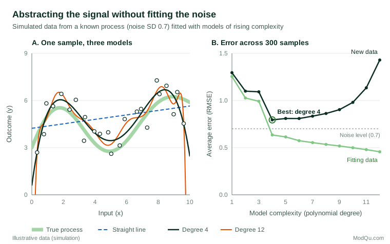
Figure 1 shows the trade-off with simulated data, where the true process is known. A straight line misses the wave in the data, with an average error on new observations of 1.29. A degree-4 polynomial captures the wave and achieves the lowest error on new data, 0.79, close to the irreducible noise level of 0.7. A degree-12 polynomial fits the original sample better still, with an error of only 0.46, but that apparent precision is false: on new data its error rises to 1.43, worse than the straight line. The model has learned the noise.
Statisticians guard against this in three main ways. Model selection criteria such as the Akaike information criterion reward fit but charge a penalty for each additional parameter (Akaike, 1974). Regularisation methods such as the lasso shrink coefficients towards zero and set many of them exactly to zero, which keeps models sparse when there are many candidate predictors (Tibshirani, 1996). Cross-validation estimates performance on data not used for fitting, the quantity shown in panel B of Figure 1.
Two cultures of modelling
Breiman (2001) distinguished two cultures in statistical modelling. The data-modelling culture assumes a stochastic model that might have generated the data and focuses on estimating its parameters. The algorithmic culture treats the mechanism as unknown and judges methods by how well they predict. Complex systems test both. Mechanistic models may be badly misspecified, while purely predictive models can fail when the system changes.
The story of Google Flu Trends illustrates the second risk. The service estimated influenza activity from search queries and was at first highly accurate. Lazer et al. (2014) showed that it later overestimated influenza substantially, at one point predicting more than double the proportion of doctor visits for influenza-like illness reported by the United States Centers for Disease Control and Prevention. They attributed the failure partly to "big data hubris" and partly to changes in the search engine itself, which altered the relationship between searches and illness. A complex system had shifted beneath a model that only tracked correlations. Businesses face the same risk whenever a demand model trained before a price change, a new competitor or a disruption to supply is used after it.
Modelling strategies for complex systems
State-space models and filtering
Many systems have a hidden state, such as true demand, brand health or economic momentum, that is observed only through noisy measurements. State-space models describe how the hidden state evolves and how observations relate to it. The Kalman (1960) filter updates the estimate of the state each time a new observation arrives, weighting it by how noisy the measurements are relative to the system. Variants of this approach underlie modern forecasting, tracking of survey indicators over time and the smoothing of noisy monthly series.
Inference by simulation
For many complex models the likelihood, the probability of the observed data given the parameters, cannot be written down or computed. Simulation offers a way around this. In approximate Bayesian computation, parameter values are drawn, the model is simulated, and values are kept when the simulated data resemble the observed data on chosen summary statistics (Beaumont et al., 2002). Wood (2010) showed that for chaotic ecological models, in which a direct likelihood behaves erratically, a synthetic likelihood based on summary statistics of simulated data allows reliable inference. The same ideas apply to agent-based models of consumers or markets.
Calibrating computer models
Large simulation models, from climate to supply-chain digital twins, must be tuned to data. Kennedy and O'Hagan (2001) set out a Bayesian framework for this calibration that explicitly includes a term for model discrepancy, the systematic gap between the simulator and reality. Treating that gap as unknown, rather than zero, prevents the calibration from forcing parameters into implausible values to compensate for missing mechanisms.
Learning structure and causation from data
Newer methods try to recover the structure of a system directly. Brunton et al. (2016) used sparse regression to identify governing equations of dynamic systems from time-series data, keeping only the few terms needed to describe the dynamics. In ecology, Sugihara et al. (2012) argued that in nonlinear coupled systems correlations can appear, vanish and even reverse over time, so correlation is an unreliable guide to causation, and they proposed convergent cross mapping as an alternative test based on how well one variable's history can reconstruct another's.
Checking models against reality
A model of a complex system should be treated as a hypothesis, not a description. Gelman and Shalizi (2013) argue that good statistical practice consists of building models, deriving their implications and checking those implications against data, revising or rejecting models that fail. Predictive checks, in which data simulated from the fitted model are compared with the observed data, are a practical way to find where a model misrepresents the system, for example by producing tails that are too thin or swings that are too regular.
Practical guidance for business and survey data
- Start simple and add complexity only when it improves performance on held-out data. A slightly worse fit to the past is often the price of a better forecast.
- Validate out of time, not only out of sample. In systems that change, test models on later periods than those used for fitting.
- Report uncertainty honestly. Prediction intervals for complex systems should be wide; narrow intervals usually mean that model uncertainty has been ignored.
- Separate sampling noise from real change. In a monthly tracking survey, a two-point movement in brand awareness may lie within sampling error. A state-space model, or a smoothed series reported with its uncertainty, helps distinguish genuine shifts from wave-to-wave noise.
- Watch for regime changes. Rising volatility or slower recovery from shocks may signal that relationships estimated in the past no longer hold (Scheffer et al., 2009).
- Combine mechanism and data. Domain knowledge about how customers, competitors and channels interact helps choose variables and constraints, while data test whether that knowledge holds.
Common mistakes
- Equating fit with knowledge. A high R² on historical data says little about whether a model has captured stable structure (Figure 1).
- Assuming normal, independent errors. Complex systems often produce heavy tails and clustered shocks, which make standard intervals too narrow (Cont, 2001).
- Trusting correlations in feedback systems. Relationships between variables in nonlinear systems can change sign over time (Sugihara et al., 2012).
- Forgetting that the system can change. Platforms, regulations and consumer habits evolve, and a model that ignores this will fail silently (Lazer et al., 2014).
Key takeaways
Statistical modelling of complex systems is the disciplined search for stable structure in noisy, interacting and changing data. Good models are deliberately simplified, chosen for their performance on new data rather than their fit to the past, and checked against reality. Tools such as regularisation, state-space filtering, simulation-based inference and calibrated simulators extend what can be learned, but none removes the need for humility: in complex systems, the most valuable knowledge often includes a clear statement of what cannot be predicted.
References
Akaike, H. (1974). A new look at the statistical model identification. IEEE Transactions on Automatic Control, 19(6), 716–723. https://doi.org/10.1109/TAC.1974.1100705
Anderson, P. W. (1972). More is different. Science, 177(4047), 393–396. https://doi.org/10.1126/science.177.4047.393
Beaumont, M. A., Zhang, W., & Balding, D. J. (2002). Approximate Bayesian computation in population genetics. Genetics, 162(4), 2025–2035. https://doi.org/10.1093/genetics/162.4.2025
Box, G. E. P. (1976). Science and statistics. Journal of the American Statistical Association, 71(356), 791–799. https://doi.org/10.1080/01621459.1976.10480949
Breiman, L. (2001). Statistical modeling: The two cultures (with comments and a rejoinder by the author). Statistical Science, 16(3), 199–231. https://doi.org/10.1214/ss/1009213726
Brunton, S. L., Proctor, J. L., & Kutz, J. N. (2016). Discovering governing equations from data by sparse identification of nonlinear dynamical systems. Proceedings of the National Academy of Sciences, 113(15), 3932–3937. https://doi.org/10.1073/pnas.1517384113
Cont, R. (2001). Empirical properties of asset returns: Stylized facts and statistical issues. Quantitative Finance, 1(2), 223–236. https://doi.org/10.1080/713665670
Gelman, A., & Shalizi, C. R. (2013). Philosophy and the practice of Bayesian statistics. British Journal of Mathematical and Statistical Psychology, 66(1), 8–38. https://doi.org/10.1111/j.2044-8317.2011.02037.x
Kalman, R. E. (1960). A new approach to linear filtering and prediction problems. Journal of Basic Engineering, 82(1), 35–45. https://doi.org/10.1115/1.3662552
Kennedy, M. C., & O'Hagan, A. (2001). Bayesian calibration of computer models. Journal of the Royal Statistical Society Series B: Statistical Methodology, 63(3), 425–464. https://doi.org/10.1111/1467-9868.00294
Lazer, D., Kennedy, R., King, G., & Vespignani, A. (2014). The parable of Google Flu: Traps in big data analysis. Science, 343(6176), 1203–1205. https://doi.org/10.1126/science.1248506
Lorenz, E. N. (1963). Deterministic nonperiodic flow. Journal of the Atmospheric Sciences, 20(2), 130–141. https://doi.org/10.1175/1520-0469(1963)020<0130:DNF>2.0.CO;2
Scheffer, M., Bascompte, J., Brock, W. A., Brovkin, V., Carpenter, S. R., Dakos, V., Held, H., van Nes, E. H., Rietkerk, M., & Sugihara, G. (2009). Early-warning signals for critical transitions. Nature, 461(7260), 53–59. https://doi.org/10.1038/nature08227
Sugihara, G., May, R., Ye, H., Hsieh, C.-h., Deyle, E., Fogarty, M., & Munch, S. (2012). Detecting causality in complex ecosystems. Science, 338(6106), 496–500. https://doi.org/10.1126/science.1227079
Tibshirani, R. (1996). Regression shrinkage and selection via the lasso. Journal of the Royal Statistical Society Series B: Statistical Methodology, 58(1), 267–288. https://doi.org/10.1111/j.2517-6161.1996.tb02080.x
Wood, S. N. (2010). Statistical inference for noisy nonlinear ecological dynamic systems. Nature, 466(7310), 1102–1104. https://doi.org/10.1038/nature09319