
Statistics · Tests and models
Quantile Regression for Distributional Knowledge Beyond Mean Effects
How quantile regression shows what drives low, typical and high values of an outcome, why that matters for spending, prices and service times, and how to fit and report it well.
Most regression analysis answers one question: how does the average outcome change when a predictor changes? For many business decisions, the average is not the most important part of the picture. A retailer cares about its heaviest spenders as much as its typical ones. A contact centre is judged on the slowest 10% of calls, not the mean waiting time. A pricing team wants to know whether a promotion lifts small baskets, large baskets or both.
Quantile regression answers these questions directly. Instead of modelling the conditional mean, it models conditional quantiles: the median, the 10th percentile, the 90th percentile or any other point of the outcome's distribution. Introduced by Koenker and Bassett (1978), it has become a standard method in economics, ecology, medicine and market research, because it shows how predictors shift and stretch an entire distribution rather than just its centre (Koenker & Hallock, 2001).
From means to quantiles
A quantile divides a distribution at a given proportion. The 0.9 quantile, or 90th percentile, of monthly spending is the amount that 90% of customers spend less than. In a sample, quantiles are easy to compute, although statistical packages use several slightly different definitions for small samples (Hyndman & Fan, 1996).
Ordinary least squares regression finds the line that minimises the sum of squared residuals, and the result estimates the conditional mean. Koenker and Bassett (1978) showed that a different loss function produces a conditional quantile instead. For the quantile τ (tau), each residual u is weighted asymmetrically:
ρτ(u) = u × (τ − I(u < 0))
Here I(u < 0) equals 1 when the observation lies below the line and 0 otherwise. For the median (τ = 0.5), positive and negative residuals count equally, and the method minimises the sum of absolute deviations. For τ = 0.9, observations above the line receive weight 0.9 and those below receive weight 0.1, so the fitted line settles where about 90% of observations lie below it. The model itself looks familiar:
Qτ(y | x) = β0(τ) + β1(τ)x1 + … + βk(τ)xk
The difference is that every coefficient carries the index τ. Fitting the model for many values of τ gives a set of coefficients for each predictor, which Koenker (2005) calls the quantile regression process. If all the slopes are the same, the predictor shifts the whole distribution up or down. If they differ, the predictor changes its spread or shape.
Why use quantile regression?
There are four main reasons to prefer quantile regression, or to use it alongside a model for the mean.
- Effects differ across the distribution. The mean can hide opposite movements in the tails. A discount might raise spending among light buyers while leaving heavy buyers unchanged, and a single average effect would understate the first and overstate the second.
- Unequal spread is the finding, not a nuisance. In ordinary regression, variance that grows with a predictor (heteroscedasticity) is treated as a problem for standard errors. In quantile regression, it is information. Cade and Noon (2003) showed in ecological data that when unmeasured factors limit a response, the upper quantiles can reveal relationships that the mean conceals.
- Robustness to extreme outcomes. The median regression line, like the sample median, is not dragged around by a few very large values in the outcome. This suits skewed business data such as order values, claim amounts and incomes.
- Invariance to monotone transformations. The 90th percentile of log spending is the log of the 90th percentile of spending. Quantile models can therefore be fitted on a transformed scale and converted back exactly, which is not true of mean models (Koenker, 2005).
A worked example: grocery spending and income
Suppose a hypothetical survey of 1,200 households records monthly grocery spending and household income. Mean spending is $158 and median spending is $143, so the distribution is skewed to the right. As Figure 1 shows, spending also fans out as income rises: lower-income households cluster tightly, while higher-income households range from modest to very high spenders.
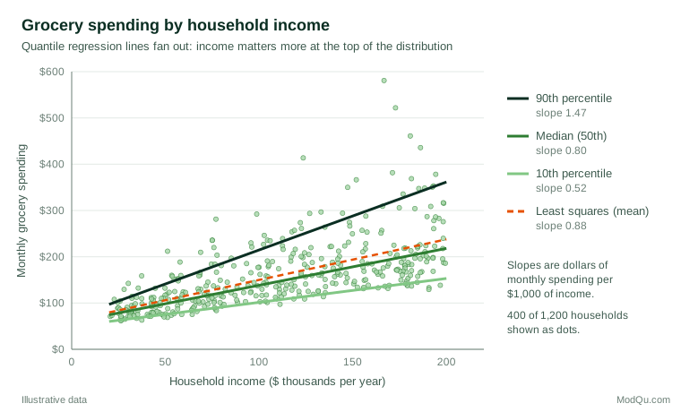
A least squares regression gives a slope of 0.88 (95% confidence interval 0.82 to 0.94): on average, each additional $10,000 of income is associated with $8.80 more monthly grocery spending. Quantile regression tells a richer story:
| Quantile of spending | Slope ($ per $1,000 income) | 95% confidence interval | Extra spending per $10,000 income |
|---|---|---|---|
| 10th percentile | 0.52 | 0.48 to 0.55 | $5.20 |
| Median | 0.80 | 0.75 to 0.85 | $8.00 |
| 90th percentile | 1.47 | 1.35 to 1.59 | $14.70 |
| Least squares (mean) | 0.88 | 0.82 to 0.94 | $8.80 |
The effect of income on high spenders is almost three times its effect on low spenders, and the confidence intervals do not overlap. In practical terms, the predicted gap between the 10th and 90th percentiles of spending is about $65 for households earning $50,000 and about $161 for households earning $150,000. A marketing team targeting high-value baskets in affluent areas would draw very different conclusions from the quantile results than from the average slope alone.
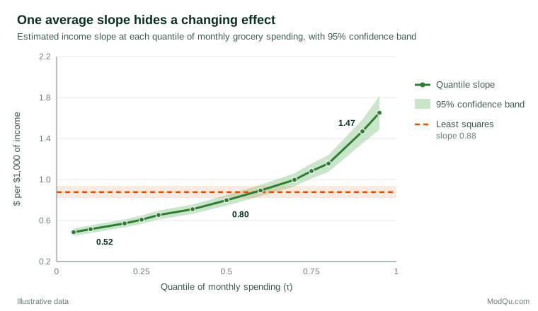
Figure 2 plots the income slope across the whole range of quantiles, the most informative single display of a quantile regression. The steady rise shows that income stretches the upper tail of spending rather than simply shifting the distribution.
Interpreting quantile coefficients correctly
The most common misreading is to treat a quantile coefficient as the effect for the people who are at that quantile. The 90th percentile slope of 1.47 describes how the 90th percentile of spending changes across income levels. It does not say that each high spender would increase spending by $14.70 if their income rose by $10,000, because households need not keep the same rank in the distribution when their circumstances change. Quantile regression describes how conditional distributions differ, not how individuals respond, unless strong additional assumptions are made.
A second subtlety concerns conditional and unconditional quantiles. Ordinary quantile regression estimates conditional quantiles: the 90th percentile of spending among households with a given income and the same values of other predictors. With several predictors, a coefficient does not describe how the overall, population-wide 90th percentile would change. Firpo et al. (2009) developed unconditional quantile regression for that question, which is often what policy and business audiences actually want to know. Machado and Mata (2005) showed how to build counterfactual distributions from quantile regressions to decompose changes in wage distributions, an approach that transfers well to comparisons of customer segments or survey waves.
Finally, a linear quantile model is an approximation. Angrist et al. (2006) showed that, even when the true conditional quantile function is not linear, quantile regression still provides a well-defined best linear approximation to it, much as least squares does for the conditional mean. Interpretation should acknowledge that approximation when the relationship is clearly curved.
Fitting, inference and model checking
Quantile regression is fitted by linear programming, which is fast even for large data sets. Inference needs more care than in least squares, because standard errors depend on the density of the outcome near the quantile in question. Common options are rank-based intervals, sandwich estimators and resampling. The bootstrap (Efron, 1979) is widely used, and Buchinsky (1998) offers practical guidance on choosing among these methods in applied work. Parzen et al. (1994) proposed a resampling method based on estimating functions that is well suited to quantile regression. Expect wider intervals in the tails: as Figure 2 shows, the 95th percentile slope is far less precise than the median slope, because fewer observations inform it.
For goodness of fit, Koenker and Machado (1999) proposed a measure analogous to R², comparing the weighted absolute residuals of the full model with those of a model containing only an intercept, together with tests of whether coefficients are equal across quantiles. Such tests answer the practical question: does a predictor really change the shape of the distribution, or only its location?
When separate quantile lines are fitted independently, they can occasionally cross, producing the impossible result that a predicted 90th percentile lies below the predicted 80th. Crossing usually appears at the edges of the data or with small samples. Chernozhukov et al. (2010) showed that rearranging the estimated quantile curves removes crossing and can only improve the estimates. For forecasting, the quantile loss above is a proper scoring rule, so it can be used to evaluate predictive quantiles fairly (Gneiting & Raftery, 2007).
Other business applications
The same logic applies wherever the tails of a distribution carry the business risk or the business opportunity.
- Service times. A contact centre can model the 50th and 90th percentiles of call-handling time against staffing levels, time of day and call type. A change that barely moves the median but sharply cuts the 90th percentile may be exactly what a service-level agreement requires.
- Prices paid and willingness to pay. In pricing surveys, stated willingness to pay is usually skewed and varies more among some segments than others. Quantile regression shows whether a product feature raises the price that the most enthusiastic tenth of buyers would accept, or only the price at the middle of the market.
- Satisfaction and experience scores. For continuous indices built from many survey items, the lower quantiles identify the drivers of very poor experiences, which are often different from the drivers of average satisfaction.
- Customer value. Spending, margin and visit frequency are typically concentrated in a minority of customers, so the upper quantiles matter most for revenue planning.
Practical guidance for survey and business data
- Choose quantiles that match decisions. Service-level targets suggest the 90th or 95th percentile of waiting time; credit or fraud reviews may focus on upper tails of exposure; pricing studies may use the quartiles. Fitting a grid such as 0.1 to 0.9 and plotting the slopes, as in Figure 2, is the best way to see the whole pattern.
- Make sure the tails have data. Extreme quantiles need large samples. A survey of 300 respondents gives only about 15 observations above the 95th percentile, too few for a reliable slope.
- Respect the survey design. Weighted and clustered surveys need weights in the estimation and design-based standard errors, for example through replicate weights (Lumley, 2010). Francisco and Fuller (1991) set out the theory for estimating quantiles under a complex survey design.
- Present predicted quantiles, not only slopes. Statements such as "for households earning $150,000, the top 10% spend more than about $288 a month" are easier to act on than coefficients.
- Use it alongside, not instead of, the mean model. The mean remains the right target for totals, such as forecast revenue. Quantile regression adds the distributional detail.
Extensions and alternatives
Quantile regression has been extended in many directions. Nonparametric and machine-learning versions relax the linear form: quantile regression forests, for example, estimate full conditional distributions from many decision trees (Meinshausen, 2006). Parametric alternatives model the distribution directly. The LMS method of Cole and Green (1992), developed for growth reference charts, and the broader generalised additive models for location, scale and shape (Rigby & Stasinopoulos, 2005) let the mean, spread and skewness all depend on predictors, giving smooth, non-crossing centile curves at the cost of stronger assumptions. For applied social scientists, Hao and Naiman (2007) give an accessible introduction to these choices and to the interpretation of quantile effects.
Common mistakes
- Reading conditional effects as individual effects, as explained above.
- Splitting the sample by the outcome (for example, running ordinary regression only on "high spenders") instead of fitting quantile regression. Selecting on the outcome biases the results; quantile regression uses all observations.
- Reporting only the median. Median regression is useful and robust, but the value of the method lies in comparing quantiles.
- Over-interpreting extreme quantiles with small samples and wide intervals.
- Ignoring crossing or survey design in published estimates.
Key takeaways
Quantile regression models the full conditional distribution of an outcome, not just its mean. It reveals predictors that stretch or compress a distribution, handles skewed and outlier-prone data well, and links naturally to business targets defined by percentiles, such as service levels or high-value customers. Interpret its coefficients as changes in conditional quantiles rather than individual responses, plot slopes across many quantiles, use appropriate standard errors and design weights, and report results as predicted quantiles that decision-makers can use.
References
Angrist, J., Chernozhukov, V., & Fernández-Val, I. (2006). Quantile regression under misspecification, with an application to the U.S. wage structure. Econometrica, 74(2), 539–563. https://doi.org/10.1111/j.1468-0262.2006.00671.x
Buchinsky, M. (1998). Recent advances in quantile regression models: A practical guideline for empirical research. The Journal of Human Resources, 33(1), 88–126. https://doi.org/10.2307/146316
Cade, B. S., & Noon, B. R. (2003). A gentle introduction to quantile regression for ecologists. Frontiers in Ecology and the Environment, 1(8), 412–420. https://doi.org/10.1890/1540-9295(2003)001[0412:AGITQR]2.0.CO;2
Chernozhukov, V., Fernández-Val, I., & Galichon, A. (2010). Quantile and probability curves without crossing. Econometrica, 78(3), 1093–1125. https://doi.org/10.3982/ECTA7880
Cole, T. J., & Green, P. J. (1992). Smoothing reference centile curves: The LMS method and penalized likelihood. Statistics in Medicine, 11(10), 1305–1319. https://doi.org/10.1002/sim.4780111005
Efron, B. (1979). Bootstrap methods: Another look at the jackknife. The Annals of Statistics, 7(1), 1–26. https://doi.org/10.1214/aos/1176344552
Firpo, S., Fortin, N. M., & Lemieux, T. (2009). Unconditional quantile regressions. Econometrica, 77(3), 953–973. https://doi.org/10.3982/ECTA6822
Francisco, C. A., & Fuller, W. A. (1991). Quantile estimation with a complex survey design. The Annals of Statistics, 19(1), 454–469. https://doi.org/10.1214/aos/1176347993
Gneiting, T., & Raftery, A. E. (2007). Strictly proper scoring rules, prediction, and estimation. Journal of the American Statistical Association, 102(477), 359–378. https://doi.org/10.1198/016214506000001437
Hao, L., & Naiman, D. Q. (2007). Quantile regression. Sage. https://doi.org/10.4135/9781412985550
Hyndman, R. J., & Fan, Y. (1996). Sample quantiles in statistical packages. The American Statistician, 50(4), 361–365. https://doi.org/10.1080/00031305.1996.10473566
Koenker, R. (2005). Quantile regression. Cambridge University Press. https://doi.org/10.1017/CBO9780511754098
Koenker, R., & Bassett, G., Jr. (1978). Regression quantiles. Econometrica, 46(1), 33–50. https://doi.org/10.2307/1913643
Koenker, R., & Hallock, K. F. (2001). Quantile regression. Journal of Economic Perspectives, 15(4), 143–156. https://doi.org/10.1257/jep.15.4.143
Koenker, R., & Machado, J. A. F. (1999). Goodness of fit and related inference processes for quantile regression. Journal of the American Statistical Association, 94(448), 1296–1310. https://doi.org/10.1080/01621459.1999.10473882
Lumley, T. (2010). Complex surveys: A guide to analysis using R. Wiley. https://doi.org/10.1002/9780470580066
Machado, J. A. F., & Mata, J. (2005). Counterfactual decomposition of changes in wage distributions using quantile regression. Journal of Applied Econometrics, 20(4), 445–465. https://doi.org/10.1002/jae.788
Meinshausen, N. (2006). Quantile regression forests. Journal of Machine Learning Research, 7, 983–999.
Parzen, M. I., Wei, L. J., & Ying, Z. (1994). A resampling method based on pivotal estimating functions. Biometrika, 81(2), 341–350. https://doi.org/10.1093/biomet/81.2.341
Rigby, R. A., & Stasinopoulos, D. M. (2005). Generalized additive models for location, scale and shape. Journal of the Royal Statistical Society Series C: Applied Statistics, 54(3), 507–554. https://doi.org/10.1111/j.1467-9876.2005.00510.x