
Statistics · Tests and models
Generalized Linear Models and Their Extensions for Diverse Outcome Types
How generalised linear models handle counts, yes/no answers, proportions, ratings and skewed spending in one framework, and which extensions to use when the basic model is not enough.
Business data rarely look like the tidy, bell-shaped outcomes that ordinary least-squares regression was built for. A customer survey records whether people renewed (yes or no), how many times they visited a store last month (0, 1, 2 and so on), what share of their grocery budget went to one retailer (a proportion between 0 and 1), how they rate a service on a five-point scale, and how much they spent (positive, and heavily skewed to the right). Each of these outcome types breaks at least one assumption of the linear model.
The generalised linear model (GLM) is the standard answer. Introduced by Nelder and Wedderburn (1972), it showed that linear regression, logistic regression, Poisson regression and several other models are special cases of a single framework, fitted with a single algorithm. Half a century later, the GLM and its extensions are the working toolkit for analysing survey and customer data. This article explains how the framework works, how to choose a model for a given outcome, how to check it, and which extensions to reach for when the basic model is not enough.
Why the linear model is not enough
Ordinary linear regression assumes that the outcome is continuous, that it can take any value, and that its spread around the fitted line is the same everywhere. Those assumptions fail for most business outcomes, in three recurring ways.
First, the range is restricted. A probability must stay between 0 and 1, a count cannot be negative, and spending cannot fall below zero. A straight line ignores those limits and will eventually predict impossible values, such as a renewal probability of 115% or −0.4 store visits.
Second, the spread depends on the mean. Customers who average one visit a month cannot vary much; customers who average ten visits can vary a great deal. When variance grows with the mean, the equal-variance assumption fails, and standard errors from ordinary regression become unreliable.
Third, effects are often multiplicative rather than additive. A loyalty programme is more plausibly described as raising visit rates by 30% than as adding exactly 0.7 visits for everyone, whether they are frequent or occasional shoppers.
A common workaround is to transform the outcome, for example by analysing the logarithm of spending, and then to fit a linear model. Transformation can help (Box & Cox, 1964 is the classic treatment), but it changes the question: the model then describes the mean of the log, not the log of the mean, and converting predictions back to the original scale is not straightforward. Manning and Mullahy (2001) compared log-transformed least squares with GLMs for skewed outcomes such as health care costs and showed that neither approach is best in every situation; the right choice depends on the shape of the residuals and on how their variance changes. GLMs avoid the retransformation problem altogether by modelling the mean on its original scale.
The three components of a generalised linear model
Every GLM is built from three parts (McCullagh & Nelder, 1989).
- A random component: a probability distribution for the outcome, chosen from the exponential family. The normal, binomial, Poisson, gamma and inverse Gaussian distributions all belong to it.
- A linear predictor: a weighted sum of the explanatory variables, exactly as in ordinary regression.
- A link function: a smooth, monotone function g that connects the mean of the outcome, μ, to the linear predictor.
g(μ) = η = β0 + β1x1 + β2x2 + … + βkxk
The link function keeps predictions in the right range. The log link, log(μ) = η, guarantees a positive mean, because μ = eη can never be negative. The logit link, log(μ ÷ (1 − μ)) = η, guarantees a probability between 0 and 1, which is why logistic regression, first set out for binary sequences by Cox (1958), fits naturally in the family. The identity link, μ = η, returns ordinary linear regression.
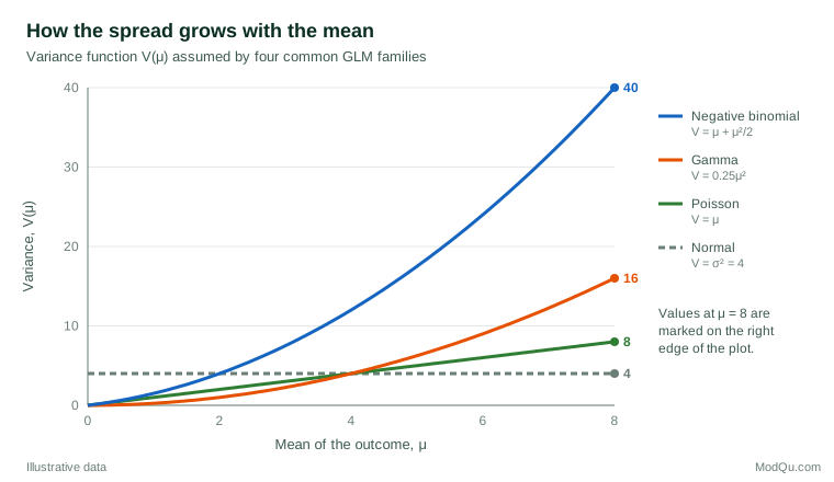
The distribution brings with it a variance function, V(μ), which states how the variance changes with the mean. For a normal outcome, the variance is constant. For a Poisson count, the variance equals the mean. For a gamma outcome, such as spending, the standard deviation is proportional to the mean, so the variance grows with its square. Figure 1 shows these patterns. Choosing a family is therefore mostly a decision about how spread behaves, not only about the shape of a histogram.
Choosing a family and link for common outcome types
The table below matches typical survey and business outcomes with a starting model. These are defaults rather than rules; the diagnostic checks described later decide whether a model is adequate.
| Outcome type | Business example | Usual family | Usual link | Effects reported as |
|---|---|---|---|---|
| Continuous, symmetric | Satisfaction index averaged over many items | Normal | Identity | Differences in means |
| Binary | Renewed, purchased, recommended | Binomial | Logit | Odds ratios, probabilities |
| Count | Store visits, complaints, page views | Poisson or negative binomial | Log | Rate ratios |
| Proportion of a known total | Coupons redeemed out of coupons sent | Binomial | Logit | Odds ratios |
| Positive, right-skewed | Spending, claim size, time to resolve | Gamma | Log | Ratios of means |
| Ordered categories | Five-point rating | Cumulative logit | Logit | Cumulative odds ratios |
| Unordered categories | Preferred brand among four | Multinomial | Logit | Relative risk ratios |
With a log link, an exponentiated coefficient is a ratio. A coefficient of 0.30 on a yes/no variable means the expected outcome is e0.30 ≈ 1.35 times higher, or 35% higher, in the "yes" group, holding the other variables constant. With a logit link, the exponentiated coefficient is an odds ratio, which is easy to misread as a ratio of probabilities (Hosmer et al., 2013). ModQu's article on logistic regression covers that case in detail.
Counts also often need an offset. When customers are observed for different lengths of time, or stores have different numbers of visitors, the model should describe a rate, such as complaints per thousand transactions. Including the logarithm of the exposure as a term with a coefficient fixed at 1 does exactly that.
Estimation, deviance and model checking
GLMs are fitted by maximum likelihood. Nelder and Wedderburn (1972) showed that the estimates can be found by iteratively reweighted least squares: the algorithm repeatedly fits a weighted linear regression to a working version of the outcome, updating the weights from the current variance function until the estimates settle. Every major statistical package uses this approach or a close relative of it.
The main measure of fit is the deviance, which compares the fitted model with a "saturated" model that reproduces every observation exactly. Differences in deviance between nested models give likelihood-ratio tests of whether added variables improve the fit. For comparing non-nested models, such as a Poisson model with a negative binomial one, information criteria are more useful; the Akaike information criterion (AIC) rewards fit and penalises the number of parameters (Akaike, 1974).
Model checking follows the same logic as in linear regression, with adapted tools (Dunn & Smyth, 2018):
- Residual plots. Deviance or Pearson residuals plotted against fitted values and each predictor should show no trend and roughly constant spread. For discrete outcomes, raw residual plots show stripes that are hard to read; randomised quantile residuals remove them.
- The dispersion statistic. The sum of squared Pearson residuals divided by the residual degrees of freedom should be close to 1 for Poisson and binomial models. Values well above 1 signal overdispersion.
- Influential observations. A handful of extreme customers, such as a corporate account with 300 visits, can drive a count model. Check leverage and influence measures, not only residuals.
- Predictive checks. Compare predicted and observed frequencies, as in the worked example below. A model that reproduces the mean but not the distribution can give misleading answers to questions such as "what share of customers never visit?"
A worked example: counting store visits
Suppose a hypothetical retailer surveys 2,000 loyalty-database customers and asks how many times each visited a store in the last month. The sample mean is 2.4 visits, but the variance is 7.8, more than three times the mean. More than a quarter of customers (28.6%) made no visit at all, and a small group visited ten times or more.
A Poisson regression is the natural first model for counts. With only the mean to work with, however, a Poisson distribution with mean 2.4 predicts just 9.1% zero visits, peaks at two visits and almost never produces customers with eight or more visits (Figure 2). The data are overdispersed: there is more variation between customers than the Poisson distribution allows. The Pearson dispersion statistic from the Poisson regression in this illustration is about 2.9, which means its standard errors are understated by a factor of roughly √2.9 ≈ 1.7. Predictors would appear far more significant than they are.
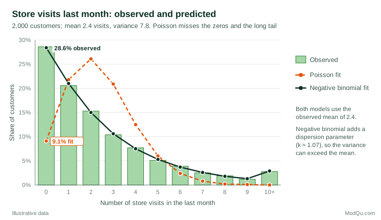
The negative binomial model adds a dispersion parameter, k, so that the variance becomes μ + μ²/k. With k ≈ 1.07, it reproduces the observed distribution closely, including 28.4% zeros against 28.6% observed. Fitted with a log link and two predictors, the hypothetical model is:
log(μ) = 0.70 + 0.30 × loyalty member − 0.08 × distance to store (km)
The exponentiated coefficients are rate ratios. Loyalty members are expected to make e0.30 ≈ 1.35 times as many visits as non-members at the same distance, and each extra kilometre reduces expected visits by about 8% (e−0.08 ≈ 0.92). For a customer living 5 km from the store, the model predicts e0.30 ≈ 1.35 visits for a non-member and e0.60 ≈ 1.82 for a member. Presenting such predicted values for typical customers is usually clearer for decision-makers than presenting coefficients on the log scale.
Overdispersion, excess zeros and how to handle them
Overdispersion is the norm rather than the exception in customer counts, because customers differ in ways no survey fully measures. Three remedies are widely used (Cameron & Trivedi, 2013).
Quasi-Poisson models keep the Poisson mean structure but estimate a dispersion factor and inflate the standard errors accordingly. They rest on quasi-likelihood, which Wedderburn (1974) showed requires only the relationship between mean and variance, not a full probability distribution. Negative binomial regression adds a parameter that lets the variance grow with the square of the mean, as in Figure 1 (Hilbe, 2011). The two approaches can give different coefficients because they weight observations differently: the quasi-Poisson model gives relatively more weight to large counts. Ver Hoef and Boveng (2007) explain the difference and recommend examining how the variance actually changes with the mean before choosing between them.
Sometimes the zeros come from a different process. Some customers do not visit because they live elsewhere or have switched retailer; they are structural non-users, not occasional shoppers who happened to skip a month. Two families of models address this. Zero-inflated models, introduced by Lambert (1992) for defects in manufacturing, mix a point mass at zero with a count distribution, so that a zero can come from either source. Hurdle models, set out by Mullahy (1986), separate the decision to visit at all from the number of visits among those who do. In market research, the hurdle structure often matches the business question well: "who shops with us?" and "how often do they shop?" are different questions with different drivers.
Excess zeros are not automatically a reason for zero-inflation. A negative binomial model often reproduces many zeros on its own, as the worked example shows. Compare candidate models with AIC and with predicted-versus-observed frequency tables before adding complexity.
Extensions for other outcome types
The GLM framework has grown into a family of related models. The most useful for business and survey data are summarised below.
Ordered and unordered categories
Rating scales are ordered but not truly numeric. The proportional odds model (McCullagh, 1980) models the cumulative probability of answering at or below each category with a common set of coefficients, giving one odds ratio per predictor. Agresti (2010) describes this and related ordinal models in depth, including checks for the proportional-odds assumption. For unordered choices, such as a preferred brand among several, the multinomial logit model estimates a set of coefficients for each category relative to a reference category.
Proportions, shares and rates
When the outcome is a proportion of a known number of trials, such as coupons redeemed out of coupons sent, binomial regression applies directly. Shares without a natural count, such as the share of wallet spent with one retailer, are harder. Fractional logit models, proposed by Papke and Wooldridge (1996) for 401(k) plan participation rates, use a logit link with quasi-likelihood estimation and handle exact zeros and ones. Beta regression (Ferrari & Cribari-Neto, 2004) assumes a beta distribution for proportions strictly between 0 and 1 and models both mean and precision.
Skewed spending and semicontinuous outcomes
Positive, right-skewed outcomes such as order values usually suit a gamma GLM with a log link. Spending in survey data is often semicontinuous: many respondents spent nothing, and the rest spent amounts that vary widely. Two-part models, which combine a logistic model for "any spending" with a gamma model for the amount, or the Tweedie family, which handles a mass at zero together with a continuous positive part in a single model, are standard options (Dunn & Smyth, 2018).
Clustered and repeated data
Survey respondents are often grouped, for example customers within stores or repeated waves of a panel. Ignoring that structure understates uncertainty. Generalised estimating equations (GEE), introduced by Liang and Zeger (1986), estimate population-average effects and give standard errors that remain valid even when the assumed within-cluster correlation is wrong. Generalised linear mixed models add random effects to the linear predictor, giving cluster-specific estimates; Breslow and Clayton (1993) developed approximate inference for this class. The two answer subtly different questions: GEE describes the average customer response across the population, while mixed models describe the response within a given store or person.
Non-linear effects and models for the whole distribution
A GLM assumes that each predictor acts linearly on the link scale. Generalised additive models (GAMs) replace linear terms with smooth functions estimated from the data (Hastie & Tibshirani, 1986). Modern implementations choose the smoothness automatically by penalised regression splines (Wood, 2017), which makes GAMs practical for curved relationships such as the effect of age or tenure on spending. Going further, generalised additive models for location, scale and shape (GAMLSS) let the variance, skewness and other features of the distribution depend on predictors too (Rigby & Stasinopoulos, 2005). These are useful when the business question concerns spread or extremes, a theme continued in ModQu's article on quantile regression.
Practical guidance for survey and business data
- Start from the outcome, not the software default. Look at the histogram, the range and the relation between group means and variances before choosing a family. Figure 1 is a useful mental checklist.
- Use design-based estimation for complex samples. When survey data are weighted, stratified or clustered, coefficients should be estimated with the survey weights and standard errors should reflect the design. Binder (1983) set out the theory for estimators defined by estimating equations, which includes GLMs, and Lumley (2010) shows how to fit survey-weighted GLMs in practice.
- Report effects on the scale people understand. Translate log-link coefficients into percentage changes and logit coefficients into predicted probabilities for typical customers. Include confidence intervals.
- Use exposure offsets whenever observation periods or opportunities differ between units.
- Check the dispersion statistic for every Poisson or binomial model before reading its significance tests.
- Prefer the simplest model that passes the checks. A negative binomial model that fits well is easier to explain than a zero-inflated model whose second component nobody can interpret.
Common mistakes
- Fitting ordinary regression to counts or proportions and reporting impossible predictions, or log-transforming counts that include zeros by adding an arbitrary constant.
- Ignoring overdispersion. A Poisson model on overdispersed data can make weak effects look highly significant.
- Confusing the scales. Coefficients act on the link scale. A log-link coefficient of 0.10 is about a 10.5% change in the mean, not an increase of 0.10 units.
- Comparing coefficients across models or groups without care. In logistic and other non-linear models, coefficients depend on unobserved variation, so their size can change when unrelated variables are added. Mood (2010) shows how this misleads comparisons across models, samples and groups, and recommends average marginal effects instead.
- Adding complexity without checking. Zero-inflated, mixed and additive models each have more ways to fail. Each added layer should earn its place with better diagnostics or a clearer answer to the business question.
- Treating associations as causes. A GLM describes how the mean outcome varies with predictors. It does not show that changing a predictor would change the outcome.
Key takeaways
Generalised linear models extend regression to the outcomes that business and survey data actually produce: binary answers, counts, proportions, ratings and skewed amounts. Each model combines a distribution, a linear predictor and a link function, and the choice of distribution is chiefly a choice about how variance changes with the mean. Check dispersion, residuals and predicted frequencies, use design-based standard errors for complex samples, and report effects as ratios, percentage changes or predicted values. When the basic GLM falls short, well-established extensions handle overdispersion, excess zeros, clustered data, non-linear effects and changing spread, but each should be justified by the data and the question rather than added by default.
References
Agresti, A. (2010). Analysis of ordinal categorical data (2nd ed.). Wiley. https://doi.org/10.1002/9780470594001
Akaike, H. (1974). A new look at the statistical model identification. IEEE Transactions on Automatic Control, 19(6), 716–723. https://doi.org/10.1109/TAC.1974.1100705
Binder, D. A. (1983). On the variances of asymptotically normal estimators from complex surveys. International Statistical Review, 51(3), 279–292. https://doi.org/10.2307/1402588
Box, G. E. P., & Cox, D. R. (1964). An analysis of transformations. Journal of the Royal Statistical Society Series B: Statistical Methodology, 26(2), 211–243. https://doi.org/10.1111/j.2517-6161.1964.tb00553.x
Breslow, N. E., & Clayton, D. G. (1993). Approximate inference in generalized linear mixed models. Journal of the American Statistical Association, 88(421), 9–25. https://doi.org/10.1080/01621459.1993.10594284
Cameron, A. C., & Trivedi, P. K. (2013). Regression analysis of count data (2nd ed.). Cambridge University Press. https://doi.org/10.1017/CBO9781139013567
Cox, D. R. (1958). The regression analysis of binary sequences. Journal of the Royal Statistical Society Series B: Statistical Methodology, 20(2), 215–232. https://doi.org/10.1111/j.2517-6161.1958.tb00292.x
Dunn, P. K., & Smyth, G. K. (2018). Generalized linear models with examples in R. Springer. https://doi.org/10.1007/978-1-4419-0118-7
Ferrari, S., & Cribari-Neto, F. (2004). Beta regression for modelling rates and proportions. Journal of Applied Statistics, 31(7), 799–815. https://doi.org/10.1080/0266476042000214501
Hastie, T., & Tibshirani, R. (1986). Generalized additive models. Statistical Science, 1(3), 297–310. https://doi.org/10.1214/ss/1177013604
Hilbe, J. M. (2011). Negative binomial regression (2nd ed.). Cambridge University Press. https://doi.org/10.1017/CBO9780511973420
Hosmer, D. W., Jr., Lemeshow, S., & Sturdivant, R. X. (2013). Applied logistic regression (3rd ed.). Wiley. https://doi.org/10.1002/9781118548387
Lambert, D. (1992). Zero-inflated Poisson regression, with an application to defects in manufacturing. Technometrics, 34(1), 1–14. https://doi.org/10.2307/1269547
Liang, K.-Y., & Zeger, S. L. (1986). Longitudinal data analysis using generalized linear models. Biometrika, 73(1), 13–22. https://doi.org/10.1093/biomet/73.1.13
Lumley, T. (2010). Complex surveys: A guide to analysis using R. Wiley. https://doi.org/10.1002/9780470580066
Manning, W. G., & Mullahy, J. (2001). Estimating log models: To transform or not to transform? Journal of Health Economics, 20(4), 461–494. https://doi.org/10.1016/S0167-6296(01)00086-8
McCullagh, P. (1980). Regression models for ordinal data. Journal of the Royal Statistical Society Series B: Statistical Methodology, 42(2), 109–127. https://doi.org/10.1111/j.2517-6161.1980.tb01109.x
McCullagh, P., & Nelder, J. A. (1989). Generalized linear models (2nd ed.). Chapman and Hall. https://doi.org/10.1201/9780203753736
Mood, C. (2010). Logistic regression: Why we cannot do what we think we can do, and what we can do about it. European Sociological Review, 26(1), 67–82. https://doi.org/10.1093/esr/jcp006
Mullahy, J. (1986). Specification and testing of some modified count data models. Journal of Econometrics, 33(3), 341–365. https://doi.org/10.1016/0304-4076(86)90002-3
Nelder, J. A., & Wedderburn, R. W. M. (1972). Generalized linear models. Journal of the Royal Statistical Society Series A: General, 135(3), 370–384. https://doi.org/10.2307/2344614
Papke, L. E., & Wooldridge, J. M. (1996). Econometric methods for fractional response variables with an application to 401(k) plan participation rates. Journal of Applied Econometrics, 11(6), 619–632. https://doi.org/10.1002/(SICI)1099-1255(199611)11:6<619::AID-JAE418>3.0.CO;2-1
Rigby, R. A., & Stasinopoulos, D. M. (2005). Generalized additive models for location, scale and shape. Journal of the Royal Statistical Society Series C: Applied Statistics, 54(3), 507–554. https://doi.org/10.1111/j.1467-9876.2005.00510.x
Ver Hoef, J. M., & Boveng, P. L. (2007). Quasi-Poisson vs. negative binomial regression: How should we model overdispersed count data? Ecology, 88(11), 2766–2772. https://doi.org/10.1890/07-0043.1
Wedderburn, R. W. M. (1974). Quasi-likelihood functions, generalized linear models, and the Gauss–Newton method. Biometrika, 61(3), 439–447. https://doi.org/10.1093/biomet/61.3.439
Wood, S. N. (2017). Generalized additive models: An introduction with R (2nd ed.). Chapman and Hall/CRC. https://doi.org/10.1201/9781315370279