
Statistics · Tests and models
Diagnostic Checking and Residual Analysis in Statistical Knowledge Validation
Why a fitted model is not finished until its residuals have been examined, which plots and tests reveal problems, and how to respond when the diagnostics fail.
A fitted regression model always produces coefficients and p-values, whether or not its assumptions hold. Software does not warn that a relationship is curved, that the variance grows with the outcome or that one unusual case is steering the results. Diagnostic checking is the step that asks whether the model deserves to be believed. Box (1976) described good statistical practice as a cycle of tentative modelling and criticism, in which the analyst fits a model, looks for ways it fails and revises it. Residual analysis is the main tool for that criticism.
What residuals are
A residual is the difference between an observed value and the value the model predicts for it:
ei = yi − ŷi
If the model is adequate, residuals should behave like random noise: centred on zero, with roughly constant spread, no pattern against the fitted values or the predictors, and no dependence on the order in which data were collected. Any systematic structure left in the residuals is information the model has failed to capture.
Anscombe (1973) made the point memorably with four small data sets that share the same means, correlation and fitted regression line yet look completely different when plotted. Summary statistics cannot replace looking at the data and the residuals.
The core diagnostic plots
Most problems show up in a handful of plots.
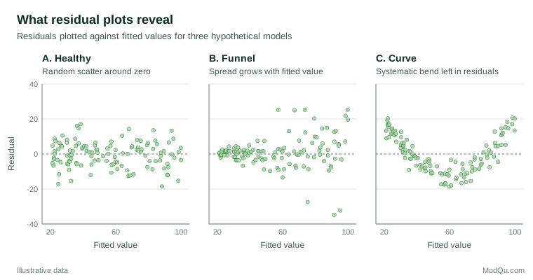
- Residuals against fitted values. The single most useful plot. A random band suggests the model is adequate; a curve suggests a missing nonlinear term; a funnel suggests non-constant variance (Figure 1).
- Residuals against each predictor, including variables left out of the model. A pattern against an omitted variable signals that it belongs in the model.
- Normal quantile plot. Points that fall along a straight line indicate approximately normal residuals; curved tails indicate skewness or heavy tails.
- Residuals in time order for data collected over days, waves or months, to reveal drift or autocorrelation.
Formal tests
Plots come first, but formal tests can confirm what the eye suspects.
- Non-constant variance. The Breusch–Pagan test regresses squared residuals on the predictors and asks whether they explain the spread (Breusch & Pagan, 1979). White (1980) proposed a related general test and, more usefully, standard errors that remain valid when the variance is not constant.
- Autocorrelation. The Durbin–Watson statistic tests whether consecutive residuals are correlated, a common issue in tracking studies and monthly sales data (Durbin & Watson, 1950).
- Normality. The Shapiro–Wilk test compares the ordered residuals with those expected under a normal distribution (Shapiro & Wilk, 1965).
Tests have a weakness in large samples: with thousands of respondents, they flag departures too small to matter. Normality in particular is often unimportant for large samples, because the central limit theorem keeps estimates of means and regression coefficients approximately normal even when the data are not (Lumley et al., 2002). Judge the size of a problem, not just its p-value.
Influential observations
Some observations affect the results far more than others. An outlier has an unusual outcome; a high-leverage point has unusual predictor values; an influential point is one whose removal would change the fitted coefficients noticeably. Cook (1977) proposed a distance measure that summarises how much all fitted values shift when a single case is deleted. Belsley et al. (1980) developed a wider set of deletion diagnostics, including measures of how much each coefficient moves. A common working rule flags cases with a Cook's distance close to or above 1, or well above the rest, for closer inspection.
A worked example
Consider a hypothetical survey of 400 households that models monthly spending on a subscription category from household income and household size. The first fit looks respectable, with a clear positive income effect. The residual plot, however, shows a funnel like Panel B in Figure 1: spending varies much more among high-income households. A Breusch–Pagan test agrees. Cook's distance also singles out one respondent with a value far above the rest; on checking, a business account had been recorded as a household.
The analyst corrects the data error and refits the model on the log of spending, which stabilises the variance and turns the income effect into a percentage change. Robust standard errors are reported as a check. The coefficients move only modestly, but the intervals for high-income groups widen to an honest size.
Practical guidance for survey and business data
- Plot before testing. Always inspect residual-versus-fitted and quantile plots; use tests as supporting evidence.
- Investigate, do not delete. An influential case may be a data error, a distinct segment or the most informative observation in the data. Report results with and without it.
- Respond to the pattern. Curvature calls for transformed or additional terms; a funnel calls for a transformation, weighted estimation or robust standard errors; autocorrelation calls for time-series methods.
- Respect the survey design. With weighted or clustered samples, use design-aware standard errors alongside diagnostics.
Common mistakes
- Checking only R². A high R² says nothing about whether the assumptions hold, as Anscombe (1973) showed.
- Testing normality of the raw outcome. The assumption concerns the residuals, not the outcome itself.
- Over-reacting to large-sample tests. Tiny departures become "significant" with big samples.
- Diagnosing once. Re-check the residuals after every revision; fixing one problem can expose another.
Key takeaways
Residual plots reveal curvature, unequal variance, dependence and unusual cases that summary statistics conceal. Formal tests and influence measures add precision, but the aim is judgement: decide whether a departure is large enough to change the conclusions, fix what can be fixed and report what remains.
References
Anscombe, F. J. (1973). Graphs in statistical analysis. The American Statistician, 27(1), 17–21. https://doi.org/10.1080/00031305.1973.10478966
Belsley, D. A., Kuh, E., & Welsch, R. E. (1980). Regression diagnostics: Identifying influential data and sources of collinearity. Wiley. https://doi.org/10.1002/0471725153
Box, G. E. P. (1976). Science and statistics. Journal of the American Statistical Association, 71(356), 791–799. https://doi.org/10.1080/01621459.1976.10480949
Breusch, T. S., & Pagan, A. R. (1979). A simple test for heteroscedasticity and random coefficient variation. Econometrica, 47(5), 1287–1294. https://doi.org/10.2307/1911963
Cook, R. D. (1977). Detection of influential observation in linear regression. Technometrics, 19(1), 15–18. https://doi.org/10.1080/00401706.1977.10489493
Durbin, J., & Watson, G. S. (1950). Testing for serial correlation in least squares regression: I. Biometrika, 37(3–4), 409–428. https://doi.org/10.2307/2332391
Lumley, T., Diehr, P., Emerson, S., & Chen, L. (2002). The importance of the normality assumption in large public health data sets. Annual Review of Public Health, 23(1), 151–169. https://doi.org/10.1146/annurev.publhealth.23.100901.140546
Shapiro, S. S., & Wilk, M. B. (1965). An analysis of variance test for normality (complete samples). Biometrika, 52(3–4), 591–611. https://doi.org/10.1093/biomet/52.3-4.591
White, H. (1980). A heteroskedasticity-consistent covariance matrix estimator and a direct test for heteroskedasticity. Econometrica, 48(4), 817–838. https://doi.org/10.2307/1912934