
Statistics · Survey statistics
Small Area Estimation
How small area estimation borrows strength from models and auxiliary data to produce reliable figures for regions, districts and subgroups where survey samples are too small for direct estimates.
National surveys are designed to give precise answers for the country as a whole and for a few large regions. Decision-makers, however, increasingly want figures for much smaller units: municipalities, postal districts, sales territories, store catchments, or narrow demographic groups. A survey of 3,000 people may include only 20 from a given district, and a percentage based on 20 interviews has a margin of error of more than 20 points. Small area estimation (SAE) is the set of statistical methods that produce usable estimates for such domains by combining the survey data with models and auxiliary information from other sources (Rao & Molina, 2015).
The term "small area" is slightly misleading. What makes an area small is the size of its sample, not its geography. A large rural region with few interviews is a small area; so is a subgroup such as women aged 18 to 24 in one province. This article explains why direct estimates fail in such domains, how the main model-based methods work, how their accuracy is measured, and how to use them responsibly in market research and business analysis.
Why direct estimates fail
A direct estimate uses only the sample data from the area itself, usually with survey weights. Design-based estimators such as the Horvitz–Thompson or generalised regression (GREG) estimator are approximately unbiased, whatever the shape of the population (Särndal et al., 1992). Their weakness is variance. With a small sample, the estimate swings widely from one possible sample to another, and some areas may have no sample at all.
The arithmetic is unforgiving. For a proportion near 50%, the 95% margin of error under simple random sampling is roughly ±98 ÷ √n percentage points, so 20 interviews give about ±22 points, 100 give about ±10, and 400 give about ±5. Real surveys are less efficient still, because clustering and weighting add a design effect, and the number of interviews that falls in a given area is itself random rather than fixed (Lohr, 2021). Areas with no sampled units at all are common when the number of areas is large: a sample of 2,000 spread across 1,000 municipalities leaves many with none.
Statistical agencies typically flag or suppress estimates whose coefficient of variation exceeds a set threshold. That protects users from unreliable figures, but it leaves exactly the local estimates that planners want blank. Increasing the sample in every area is usually unaffordable: covering 500 districts with 400 interviews each would need a survey of 200,000. SAE offers a different route. It accepts a small amount of model-based bias in exchange for a large reduction in variance, a trade-off that often reduces the overall error considerably (Ghosh & Rao, 1994).
Borrowing strength
All SAE methods rest on one idea: borrowing strength from related areas, from other time periods, or from auxiliary variables available for every area. Purcell and Kish (1979) classified the early methods into three broad families.
- Synthetic estimators assume that a relationship estimated for a large area also holds for each small area within it. If a national survey finds that product usage varies by age group, a synthetic estimate for a district applies the national rates for each age group to the district's census age profile. Synthetic estimates are stable but can be badly biased if the area differs in ways the model does not capture.
- Composite estimators take a weighted average of the direct estimate and the synthetic estimate, giving more weight to the direct estimate when the area sample is large.
- Model-based estimators formalise the composite idea through explicit statistical models, usually mixed models with random area effects. The model determines how much weight each source receives and also provides a measure of uncertainty.
Modern SAE is dominated by the third family, which links the subject to the theory of best linear unbiased prediction (BLUP) for mixed models (Henderson, 1975; Robinson, 1991) and to empirical Bayes estimation (Efron & Morris, 1975).
The area-level model: Fay–Herriot
The most widely used model was introduced by Fay and Herriot (1979) to estimate per capita income for small places in the United States, where many direct survey estimates were very imprecise. It works with area summaries only, which makes it practical when unit-level data cannot be linked to auxiliary sources.
The model has two parts. The first describes sampling error: the direct estimate for area i equals the true value plus noise with a known sampling variance ψi. The second is a linking model that relates the true values to area-level auxiliary variables, such as census or administrative data, plus a random area effect with variance σu2:
θ̂i = θi + ei, ei ~ N(0, ψi)
θi = xi′β + ui, ui ~ N(0, σu2)
The resulting estimator, the empirical best linear unbiased predictor (EBLUP), is a weighted average of the direct estimate and the regression-synthetic estimate:
θ̃i = γi θ̂i + (1 − γi) xi′β̂, where γi = σu2 ÷ (σu2 + ψi)
The shrinkage factor γi is the heart of the method. When an area's direct estimate is precise (small ψi), γi is close to 1 and the direct estimate dominates. When it is noisy, γi is close to 0 and the estimate is pulled towards the model prediction. When the model explains the areas well (small σu2), all areas lean more heavily on it. This is the same logic as the James–Stein shrinkage that Efron and Morris (1975) demonstrated with baseball batting averages: pulling individually noisy estimates towards a common prediction reduces total error.
The unit-level model: Battese–Harter–Fuller
When survey responses can be matched to auxiliary information for individual units, a unit-level model can be used. Battese et al. (1988) proposed the nested error regression model to estimate the areas planted with corn and soybeans in twelve Iowa counties, using farm survey data together with satellite counts of pixels classified as each crop:
yij = xij′β + ui + eij
Here yij is the outcome for unit j in area i, ui is the area effect and eij is the individual error. The model needs the area means of the auxiliary variables for the whole population, for example from a census, a customer database or a business register. Unit-level models usually use the information more efficiently than area-level models, but they require consistent definitions of the auxiliary variables in the survey and in the population source, and they are more sensitive to the sample design if selection depends on the outcome (Pfeffermann, 2013).
Area-level or unit-level?
The choice between the two model types is usually decided by the data rather than by preference. Area-level models need only direct estimates, their sampling variances and area-level covariates. They automatically respect the survey weights, because the direct estimates already use them, and they can draw on published aggregates when microdata cannot be linked. Their weaknesses are that the sampling variances ψi are treated as known when they are in fact estimated, often poorly, for small areas, and that areas with no sample receive only a synthetic estimate. In practice ψi is often smoothed, for example by modelling it as a function of sample size (Rao & Molina, 2015).
Unit-level models need auxiliary variables that are measured in the same way for every sampled unit and for the whole population, or at least their area means. When such data exist, for instance a customer database that covers all accounts and can be linked to survey respondents, unit-level models usually give more precise estimates and handle non-linear indicators more naturally (Molina & Rao, 2010).
Measuring accuracy
An SAE estimate is only useful if users know how accurate it is. Because model-based estimators may be biased for an individual area, accuracy is measured by the mean squared error (MSE) rather than the variance. For the Fay–Herriot model, the leading term of the MSE is γiψi, which is always smaller than the direct estimate's variance ψi. However, the model parameters β and σu2 are themselves estimated, and ignoring this extra uncertainty understates the error. Prasad and Rao (1990) derived an MSE estimator that accounts for it, and bootstrap and jackknife alternatives are now common (Jiang & Lahiri, 2006).
The MSE from a model is an average over the model's assumptions. It says how accurate estimates are on average across areas that behave like the model, not how accurate a specific area's estimate is if that area is unusual. This is why model checking is essential.
A worked example
Suppose a hypothetical telecommunications company runs a national survey and wants the share of households using a new streaming service in ten sales districts, labelled A to J. District sample sizes range from 20 to 400. For every district, the company also knows from its own records the share of households with high-speed internet, xi. The fitted Fay–Herriot model (illustrative values) is:
θi = 10 + 0.5 xi + ui, σu2 = 16 (an area-level standard deviation of 4 points)
The sampling variances ψi are based on the model-predicted proportions and an assumed design effect of 1.5.
| District | Sample | Direct estimate | 95% margin (direct) | Model prediction | γi | EBLUP | 95% margin (EBLUP) |
|---|---|---|---|---|---|---|---|
| A | 20 | 55% | ±26.3 | 40.0% | 0.08 | 41.2% | ±7.5 |
| C | 50 | 30% | ±16.4 | 37.5% | 0.19 | 36.1% | ±7.1 |
| F | 120 | 48% | ±10.9 | 45.0% | 0.34 | 46.0% | ±6.4 |
| J | 400 | 40% | ±5.9 | 41.0% | 0.64 | 40.4% | ±4.7 |
District A illustrates the method most clearly. Its direct estimate of 55% is based on only 20 interviews and is almost useless, with a margin of ±26 points. The model gives it a weight of only 0.08, so the EBLUP of 41.2% is close to the model prediction of 40.0%. In district J, with 400 interviews, the direct estimate receives a weight of 0.64 and the EBLUP stays close to it. Figure 1 shows all ten districts. (The EBLUP margins here use only the leading MSE term γiψi; a full Prasad–Rao calculation would widen them slightly.)
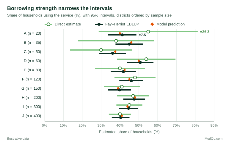
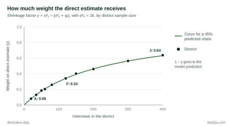
Figure 2 shows the shrinkage factors directly. The weight on the direct estimate rises with sample size but stays well below 1 even at 400 interviews, because the area effects in this example are modest relative to sampling noise.
Extensions used in practice
Poverty and welfare mapping. Elbers et al. (2003) developed a widely used method for combining a household survey with census microdata to estimate poverty and inequality for small localities. Molina and Rao (2010) proposed an empirical best approach under a unit-level model that is more efficient for non-linear indicators such as poverty rates.
Robust methods. Outlying areas or units can distort mixed-model estimates. M-quantile models (Chambers & Tzavidis, 2006) offer a robust alternative that does not depend on normally distributed random effects.
Bayesian hierarchical models. Hierarchical Bayesian models fit the same structure and give full posterior distributions for every area, which is convenient for ranking areas or computing the probability that an area exceeds a threshold (Gelman et al., 2013).
Multilevel regression and poststratification (MRP). Park et al. (2004) fitted multilevel models to national opinion polls and poststratified the predictions to census counts to produce state-level estimates. Wang et al. (2015) applied MRP to a large, highly non-representative sample of video game users and obtained election forecasts in line with those from standard polls. MRP has become a popular SAE tool in market and opinion research, although it relies heavily on the model when the sample is unrepresentative.
Time and space. Models can borrow strength across survey waves and neighbouring areas, which helps when each wave alone is thin. Pfeffermann (2002, 2013) reviews these and other developments.
A production workflow
Tzavidis et al. (2018) set out a framework for producing small area statistics that runs from specification to dissemination. It is a useful checklist for business projects as well as official statistics:
- Specify the need. Define the target indicators, the areas, and the precision users require.
- Assess the data. Check that auxiliary variables are measured consistently in the survey and in the population source, and that they are current.
- Compute direct estimates and their variances first. These are the raw material for area-level models and the benchmark for evaluating everything else.
- Build and check the model. Examine residuals, look for outlying areas, and compare model predictions with direct estimates for well-sampled areas.
- Estimate MSE with a method that accounts for parameter estimation.
- Benchmark where needed, so that area estimates add up to the reliable direct estimate for the larger region or the nation.
- Communicate the estimates, their uncertainty and their model-based nature clearly.
Software such as the sae package in R implements the main area-level and unit-level estimators, together with MSE estimation (Molina & Marhuenda, 2015).
Practical guidance for business data
- Good auxiliary data matter more than clever models. The gains from SAE come almost entirely from the strength of the relationship between the outcome and the auxiliary variables. Census profiles, customer databases, sales records and administrative registers are the usual sources.
- Validate where you can. Compare model estimates with direct estimates in areas with large samples, or with external figures where they exist. A model that cannot reproduce well-measured areas should not be trusted for poorly measured ones.
- Be clear about design-based versus model-based inference. Direct estimates rely on the sampling design; SAE estimates rely on a model being approximately correct. Little (2004) compares the two modes of inference and argues for models that respect the sample design; in practice, reporting which estimates come from which method avoids misunderstanding.
- Check for over-shrinkage before ranking areas. EBLUPs are optimal for each area individually, but as a set they are less spread out than the true values. Tables that rank districts or identify extremes should take this into account, for example by using constrained estimators designed to match the spread of the true values (Rao & Molina, 2015).
- Benchmark to trusted totals. Users notice when district figures do not add up to the published national figure. Benchmarking makes the set coherent at a small cost in precision.
Common mistakes
- Treating model estimates as survey measurements. An SAE estimate for an area with almost no sample is mostly a model prediction. It can describe the expected value for an area with those characteristics, but it cannot reveal local surprises that the auxiliary data do not capture.
- Using auxiliary data that differ from the survey definition. A "household" or "customer" defined differently in the two sources introduces bias that no model can correct.
- Ignoring the uncertainty in the model parameters. Leading-term MSE estimates understate error, especially with few areas.
- Feeding back model results as evidence for the model. If areas are later assessed against the same auxiliary variables used in the model, the agreement is built in.
- Over-interpreting differences between areas. Two districts with nearly identical EBLUPs can differ in truth, and two with different EBLUPs may differ only because their auxiliary data differ.
Key takeaways
Small area estimation produces reliable estimates for domains where survey samples are too small for direct estimates. It works by borrowing strength from auxiliary data and related areas through explicit models, most commonly the area-level Fay–Herriot model and the unit-level nested error model. The EBLUP shrinks noisy direct estimates towards model predictions, with more shrinkage where samples are smaller. Accuracy is measured by mean squared error, which must account for estimated model parameters. Used with strong auxiliary data, careful model checking, benchmarking and transparent reporting, SAE turns a national survey into credible local evidence.
References
Battese, G. E., Harter, R. M., & Fuller, W. A. (1988). An error-components model for prediction of county crop areas using survey and satellite data. Journal of the American Statistical Association, 83(401), 28–36. https://doi.org/10.1080/01621459.1988.10478561
Chambers, R., & Tzavidis, N. (2006). M-quantile models for small area estimation. Biometrika, 93(2), 255–268. https://doi.org/10.1093/biomet/93.2.255
Efron, B., & Morris, C. (1975). Data analysis using Stein's estimator and its generalizations. Journal of the American Statistical Association, 70(350), 311–319. https://doi.org/10.1080/01621459.1975.10479864
Elbers, C., Lanjouw, J. O., & Lanjouw, P. (2003). Micro-level estimation of poverty and inequality. Econometrica, 71(1), 355–364. https://doi.org/10.1111/1468-0262.00399
Fay, R. E., & Herriot, R. A. (1979). Estimates of income for small places: An application of James–Stein procedures to census data. Journal of the American Statistical Association, 74(366a), 269–277. https://doi.org/10.1080/01621459.1979.10482505
Gelman, A., Carlin, J. B., Stern, H. S., Dunson, D. B., Vehtari, A., & Rubin, D. B. (2013). Bayesian data analysis (3rd ed.). Chapman and Hall/CRC. https://doi.org/10.1201/b16018
Ghosh, M., & Rao, J. N. K. (1994). Small area estimation: An appraisal. Statistical Science, 9(1), 55–76. https://doi.org/10.1214/ss/1177010647
Henderson, C. R. (1975). Best linear unbiased estimation and prediction under a selection model. Biometrics, 31(2), 423–447. https://doi.org/10.2307/2529430
Jiang, J., & Lahiri, P. (2006). Mixed model prediction and small area estimation. TEST, 15(1), 1–96. https://doi.org/10.1007/BF02595419
Little, R. J. (2004). To model or not to model? Competing modes of inference for finite population sampling. Journal of the American Statistical Association, 99(466), 546–556. https://doi.org/10.1198/016214504000000467
Lohr, S. L. (2021). Sampling: Design and analysis (3rd ed.). Chapman and Hall/CRC. https://doi.org/10.1201/9780429298899
Molina, I., & Marhuenda, Y. (2015). sae: An R package for small area estimation. The R Journal, 7(1), 81–98. https://doi.org/10.32614/RJ-2015-007
Molina, I., & Rao, J. N. K. (2010). Small area estimation of poverty indicators. Canadian Journal of Statistics, 38(3), 369–385. https://doi.org/10.1002/cjs.10051
Park, D. K., Gelman, A., & Bafumi, J. (2004). Bayesian multilevel estimation with poststratification: State-level estimates from national polls. Political Analysis, 12(4), 375–385. https://doi.org/10.1093/pan/mph024
Pfeffermann, D. (2002). Small area estimation: New developments and directions. International Statistical Review, 70(1), 125–143. https://doi.org/10.1111/j.1751-5823.2002.tb00352.x
Pfeffermann, D. (2013). New important developments in small area estimation. Statistical Science, 28(1), 40–68. https://doi.org/10.1214/12-STS395
Prasad, N. G. N., & Rao, J. N. K. (1990). The estimation of the mean squared error of small-area estimators. Journal of the American Statistical Association, 85(409), 163–171. https://doi.org/10.1080/01621459.1990.10475320
Purcell, N. J., & Kish, L. (1979). Estimation for small domains. Biometrics, 35(2), 365–384. https://doi.org/10.2307/2530340
Rao, J. N. K., & Molina, I. (2015). Small area estimation (2nd ed.). Wiley. https://doi.org/10.1002/9781118735855
Robinson, G. K. (1991). That BLUP is a good thing: The estimation of random effects. Statistical Science, 6(1), 15–32. https://doi.org/10.1214/ss/1177011926
Särndal, C.-E., Swensson, B., & Wretman, J. (1992). Model assisted survey sampling. Springer. https://doi.org/10.1007/978-1-4612-4378-6
Tzavidis, N., Zhang, L.-C., Luna, A., Schmid, T., & Rojas-Perilla, N. (2018). From start to finish: A framework for the production of small area official statistics. Journal of the Royal Statistical Society Series A: Statistics in Society, 181(4), 927–979. https://doi.org/10.1111/rssa.12364
Wang, W., Rothschild, D., Goel, S., & Gelman, A. (2015). Forecasting elections with non-representative polls. International Journal of Forecasting, 31(3), 980–991. https://doi.org/10.1016/j.ijforecast.2014.06.001