
Statistics · Descriptive statistics
Skewness and Kurtosis: Describing the Shape of a Distribution
What skewness and kurtosis measure, how to calculate and read them, and why the shape of a distribution matters when reporting averages from survey and business data.
A mean and a standard deviation tell you where data sit and how spread out they are, but not what shape they take. Two survey questions can share the same average and spread while one has a long tail of very high values and the other is evenly balanced. Skewness and kurtosis are the two standard numbers for describing that shape. Karl Pearson developed the idea of measuring asymmetry in his work on "skew variation" (Pearson, 1895), and both measures remain routine output in statistical software.
Skewness: is the distribution lopsided?
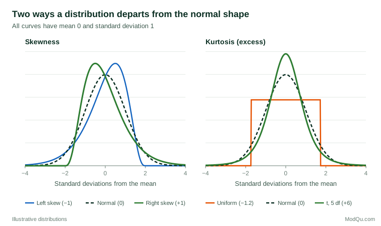
Skewness measures asymmetry around the mean. A symmetric distribution, such as the normal curve, has skewness of zero. Positive (right) skew means a long tail of high values: household income, order values and time spent on a website usually look like this. Negative (left) skew means a long tail of low values, which is common for satisfaction ratings where most customers choose the top of the scale.
The usual sample measure is based on the third moment, the average cubed deviation from the mean, scaled by the standard deviation:
g1 = m3 ÷ m23/2, where mk = (1/n) Σ (xi − x̄)k
Cubing keeps the sign of each deviation, so large values far above the mean push the result up and large values far below push it down.
Kurtosis: how heavy are the tails?
Kurtosis is based on the fourth moment. It is usually reported as excess kurtosis, the value minus 3, so that the normal distribution scores zero:
g2 = m4 ÷ m22 − 3
Positive excess kurtosis indicates heavier tails than the normal curve, meaning more extreme values; negative values indicate lighter tails. Many textbooks describe kurtosis as "peakedness", but this is misleading. Because deviations are raised to the fourth power, the measure is dominated by values far from the mean, and Westfall (2014) shows that it says very little about the peak and a great deal about the tails. Earlier reviews reached a similar view: kurtosis reflects how probability mass moves between the centre, the shoulders and the tails of a distribution (Balanda & MacGillivray, 1988; DeCarlo, 1997).
A worked example
Suppose ten respondents in a hypothetical survey report monthly spending on a service: $20, 25, 30, 30, 35, 40, 45, 50, 80 and 145. The mean is $50, but the median is only $37.50, because two high spenders pull the mean upwards. The moment formulas give skewness g1 = 1.84 and excess kurtosis g2 = 2.28, signalling a clear right tail.
Software packages do not all report the same version. Many apply small-sample adjustments, which here give skewness of 2.18 and excess kurtosis of 5.00. Joanes and Gill (1998) compare the common definitions and show that the differences are small in large samples but can be substantial in small ones, so always state which version you report. Removing the single $145 respondent cuts the adjusted skewness to 1.56 and the excess kurtosis to 3.00, which shows how strongly one extreme value can drive both measures.
Why shape matters for business data
Real data are rarely normal. Micceri (1989) examined 440 large-sample achievement and psychometric distributions and found that every one departed significantly from normality. In a study of 693 small-sample distributions, Blanca et al. (2013) found that only 5.5% were close to the values expected under normality, although extreme departures were not common. For survey analysts, this has practical consequences:
- Choose the right summary. For strongly skewed variables such as spend or income, report the median alongside the mean, or use both with a clear explanation.
- Check model assumptions. Many tests and confidence intervals assume approximate normality. Marked skewness or heavy tails may call for a transformation, robust methods or a larger sample.
- Look for data problems. Extreme kurtosis often reveals outliers, data-entry errors or a mix of distinct customer groups.
- Report shape routinely. Doane and Seward (2011) argue that skewness is underused as a descriptive statistic and discuss how to judge whether a sample value is large enough to matter.
Common mistakes
- Reading direction from mean and median alone. The textbook rule that the mean lies above the median in right-skewed data often fails, especially for discrete variables such as rating scales (von Hippel, 2005).
- Over-interpreting small samples. In large samples the standard error of skewness is roughly √(6/n) and that of kurtosis roughly √(24/n). With 10 respondents, a skewness of 1.5 is still uncertain.
- Treating kurtosis as peakedness. Describe it as tail weight or propensity for outliers.
- Ignoring the scale. On a five-point rating scale, a few categories limit how skewed or heavy-tailed the data can be, so compare shape measures only across similar scales.
Key takeaways
Skewness and kurtosis complete the description of a variable started by its mean and standard deviation. Skewness shows whether a distribution leans to one side; kurtosis shows how much weight sits in its tails. Use them to choose sensible summaries, to check assumptions behind statistical tests and to spot outliers. Always state which formula your software uses, interpret them with the sample size in mind, and pair them with a histogram.
References
Balanda, K. P., & MacGillivray, H. L. (1988). Kurtosis: A critical review. The American Statistician, 42(2), 111–119. https://doi.org/10.1080/00031305.1988.10475539
Blanca, M. J., Arnau, J., López-Montiel, D., Bono, R., & Bendayan, R. (2013). Skewness and kurtosis in real data samples. Methodology, 9(2), 78–84. https://doi.org/10.1027/1614-2241/a000057
DeCarlo, L. T. (1997). On the meaning and use of kurtosis. Psychological Methods, 2(3), 292–307. https://doi.org/10.1037/1082-989X.2.3.292
Doane, D. P., & Seward, L. E. (2011). Measuring skewness: A forgotten statistic? Journal of Statistics Education, 19(2). https://doi.org/10.1080/10691898.2011.11889611
Joanes, D. N., & Gill, C. A. (1998). Comparing measures of sample skewness and kurtosis. Journal of the Royal Statistical Society: Series D (The Statistician), 47(1), 183–189. https://doi.org/10.1111/1467-9884.00122
Micceri, T. (1989). The unicorn, the normal curve, and other improbable creatures. Psychological Bulletin, 105(1), 156–166. https://doi.org/10.1037/0033-2909.105.1.156
Pearson, K. (1895). Contributions to the mathematical theory of evolution. II. Skew variation in homogeneous material. Philosophical Transactions of the Royal Society of London (A), 186, 343–414. https://doi.org/10.1098/rsta.1895.0010
von Hippel, P. T. (2005). Mean, median, and skew: Correcting a textbook rule. Journal of Statistics Education, 13(2). https://doi.org/10.1080/10691898.2005.11910556
Westfall, P. H. (2014). Kurtosis as peakedness, 1905–2014. R.I.P. The American Statistician, 68(3), 191–195. https://doi.org/10.1080/00031305.2014.917055