
Statistics · Descriptive statistics
Percentiles, Quartiles and the Interquartile Range
What percentiles, quartiles and the interquartile range measure, why software gives different answers, how box plots and the 1.5 × IQR rule work, and how to use them with survey data.
Averages answer the question "what is typical?", but many business questions are about position. Is a customer's spend high compared with everyone else? What do the top 10% of households earn? Percentiles and quartiles answer these questions directly, and the interquartile range (IQR) gives a measure of spread that is not thrown off by a few extreme values. Together they form the backbone of exploratory data analysis (Tukey, 1977) and of the box plot, one of the most widely used charts in statistics (Krzywinski & Altman, 2014).
What a percentile is
The pth percentile is the value below which roughly p% of the observations fall. If the 90th percentile of monthly spend is $120, about 90% of customers spend less than $120 and about 10% spend more. The median is simply the 50th percentile.
More generally, statisticians speak of quantiles: the value that divides a distribution at any proportion between 0 and 1. Percentiles divide it into hundredths, deciles into tenths, quintiles into fifths and quartiles into quarters. Income statistics, for example, are often reported by quintile or decile, and paediatric growth charts plot children's height and weight against reference centile curves, a method refined by Cole and Green (1992).
A related idea is the percentile rank, which runs the other way: it takes an observed value and reports the percentage of observations at or below it. A respondent whose satisfaction score has a percentile rank of 80 scored as high as or higher than 80% of the sample. Confusing a percentile (a value) with a percentile rank (a percentage) is a common source of muddled reporting.
Quartiles and the five-number summary
The three quartiles split ordered data into four groups of roughly equal size:
- Q1, the first or lower quartile, is the 25th percentile.
- Q2 is the median, the 50th percentile.
- Q3, the third or upper quartile, is the 75th percentile.
Adding the minimum and maximum gives Tukey's five-number summary: minimum, Q1, median, Q3, maximum. Tukey (1977) proposed it as a quick, resistant description of a batch of numbers. It also reveals shape: if the median sits much closer to Q1 than to Q3, the data are skewed to the right, which is typical of spend, income and time-on-site data.
Why there is more than one way to calculate a quartile
With large samples, every sensible method gives almost the same quartiles. With small samples, they can differ noticeably, because a quartile often falls between two observations and the methods disagree about how to interpolate. Hyndman and Fan (1996) catalogued nine definitions of the sample quantile in use in statistical packages, showed that different packages used different defaults, and recommended a single standard. Langford (2006) surveyed the many competing definitions found in elementary statistics teaching.
Take a hypothetical sample of 12 respondents' monthly spend, in dollars, sorted from lowest to highest:
18, 22, 25, 27, 30, 34, 38, 41, 45, 52, 60, 140
The median is the average of the 6th and 7th values, (34 + 38) ÷ 2 = 36, on every common method. The quartiles are another matter:
| Method | Where it is used | Q1 | Q3 | IQR |
|---|---|---|---|---|
| Linear interpolation (type 7) | R and NumPy defaults; Excel QUARTILE.INC | 26.5 | 46.75 | 20.25 |
| Tukey's hinges (median of each half) | Hand calculation, many textbooks | 26.0 | 48.5 | 22.5 |
| Weibull positions (type 6) | Excel QUARTILE.EXC; SPSS and Minitab | 25.5 | 50.25 | 24.75 |
The linear method places the pth quantile at position 1 + p(n − 1) in the sorted data and interpolates between neighbouring values. For Q1 with n = 12, that is position 3.75, three-quarters of the way from 25 to 27, which gives 26.5. The Weibull method uses position p(n + 1) instead, which is 3.25 and gives 25.5. Hyndman and Fan (1996) reported type 6 as the method then used by Minitab and SPSS.
Linear (type 7): position = 1 + p(n − 1) Weibull (type 6): position = p(n + 1)
None of these answers is wrong; they are different estimates of the same population quartile. The practical lesson is to state which method was used when results matter, and to use the same method across waves of a tracking study. Harrell and Davis (1982) proposed a smoother alternative that weights all the order statistics rather than one or two, which can give more stable estimates in small samples.
The interquartile range
The interquartile range is the distance between the upper and lower quartiles:
IQR = Q3 − Q1
It covers the middle 50% of the data. In the worked example, using the linear method, the IQR is 46.75 − 26.5 = 20.25 dollars. Half of the respondents spend within a band about $20 wide, centred near the median of $36.
The main attraction of the IQR is robustness. The standard deviation of the same 12 values is about $32.6, inflated by the single respondent who spends $140; remove that one person and it falls to about $13. The IQR changes much less, from 20.25 to 17, because it ignores the top and bottom quarters of the data. Robust statistics formalises this idea through the influence a single observation can have on an estimate (Hampel, 1974) and through the breakdown point, the share of the data that can be corrupted before the estimate becomes meaningless. The IQR has a breakdown point of 25%; the median absolute deviation reaches the maximum of 50% (Rousseeuw & Croux, 1993).
For data from a normal distribution, the IQR is about 1.349 standard deviations, so IQR ÷ 1.349 is a robust estimate of the standard deviation. Rousseeuw and Croux (1993) also point out that the median absolute deviation is much less statistically efficient than the standard deviation when data really are normal, and robust measures of spread generally pay some price in efficiency for their resistance. Wilcox (2012) gives a thorough practical treatment of these trade-offs.
Box plots and the 1.5 × IQR rule
The box plot, introduced by Tukey (1977), draws the five-number summary as a picture. The box runs from Q1 to Q3, a line inside it marks the median, and whiskers extend towards the extremes. In the standard version, any point more than 1.5 × IQR beyond the box is drawn separately as a possible outlier. The two cut-offs are called fences:
Lower fence = Q1 − 1.5 × IQR Upper fence = Q3 + 1.5 × IQR
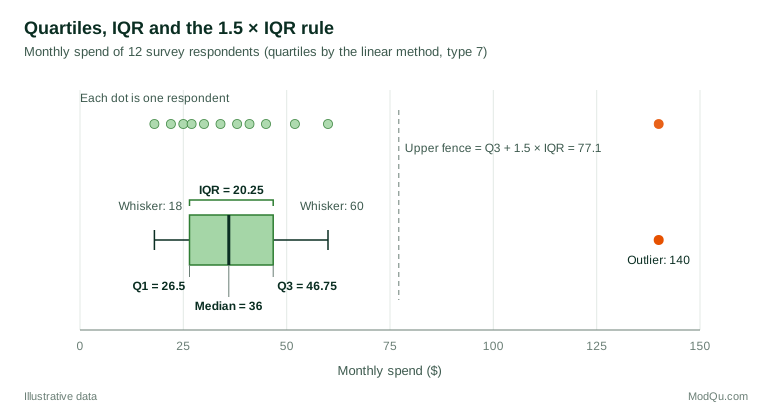
In the worked example the upper fence is 46.75 + 1.5 × 20.25 ≈ 77.1, so the respondent spending $140 is flagged. The lower fence is below zero, so nothing is flagged at the bottom. Each whisker stops at the most extreme observation still inside its fence: 18 at the bottom and 60 at the top.
For a normal population, the fences sit about 2.7 standard deviations from the mean, so roughly 0.7% of observations fall outside them. That sounds small, but in a sample of 1,000 respondents it means about seven flagged points even when the data are perfectly clean. Hoaglin et al. (1986) studied how often the rule labels outliers in well-behaved samples of different sizes, and their results show that "outside" points should be treated as candidates for checking rather than as errors to delete.
Two further cautions apply. First, software implements box plots in different ways, mainly because of the quartile definitions above, so the same data can produce different whiskers and different flagged points in different packages (Frigge et al., 1989). Second, the rule assumes rough symmetry. In strongly skewed data, such as spend or session length, it flags many legitimate high values. Hubert and Vandervieren (2008) proposed an adjusted box plot that widens the fence on the long-tailed side using a robust measure of skewness.
Box plots also have useful variants. McGill et al. (1978) added notches around the median, roughly a confidence interval, so that two boxes whose notches do not overlap suggest a real difference in medians, and variable widths that show the size of each group. Krzywinski and Altman (2014) give a concise guide to constructing and reading box plots and their variants. Reporting the sample size with every box, and overlaying the raw points when samples are small as in Figure 1, helps readers judge how much weight each box can bear.
Percentiles in survey and business data
Use weights. In a weighted survey, a percentile should be found from the weighted distribution: sort respondents by the variable, accumulate their weights, and read off the value at which the cumulative weight first reaches p% of the total (Lohr, 2021). An unweighted median from a sample that over-represents high-income households will overstate the population median.
Report uncertainty. A sample percentile is an estimate and has a margin of error. Woodruff (1952) developed a widely used method for confidence intervals for medians and other quantiles in sample surveys. Francisco and Fuller (1991) extended the theory of quantile estimation to complex survey designs. Extreme percentiles, such as the 95th or 99th, need large samples: with 200 respondents, the 99th percentile rests on the top two observations.
Choose robust screening rules. When cleaning survey data, rules based on the median and IQR or the median absolute deviation are usually safer than rules based on the mean and standard deviation, because the outliers being sought also inflate the mean and standard deviation that are meant to detect them (Leys et al., 2013).
Look beyond the average effect. Quantile regression models a chosen percentile of an outcome, such as the 10th or 90th percentile of spend, rather than its mean. It can show, for example, that a loyalty programme raises spending among heavy buyers but does little for light buyers (Koenker & Hallock, 2001).
Common mistakes
- Mixing quartile methods. Comparing quartiles calculated in different packages, or with different spreadsheet functions, can create apparent changes that are purely computational.
- Deleting every flagged point. The 1.5 × IQR rule identifies values worth checking, not values that are wrong. A respondent who really spends $140 is part of the market.
- Averaging percentiles. The median of a combined group is not the average of the group medians. Percentiles must be recalculated from the pooled, weighted data.
- Reading percentiles from tiny groups. Quartiles for a subgroup of 15 respondents are rough, and deciles are almost meaningless.
Key takeaways
Percentiles locate values within a distribution, quartiles divide it into four parts, and the interquartile range measures the spread of the middle half. These measures are simple to explain, resistant to extreme values and well suited to the skewed data common in business. Use weighted percentiles for survey data, report the calculation method and the uncertainty, and treat box plot outliers as prompts for investigation rather than automatic deletions.
References
Cole, T. J., & Green, P. J. (1992). Smoothing reference centile curves: The LMS method and penalized likelihood. Statistics in Medicine, 11(10), 1305–1319. https://doi.org/10.1002/sim.4780111005
Francisco, C. A., & Fuller, W. A. (1991). Quantile estimation with a complex survey design. The Annals of Statistics, 19(1), 454–469. https://doi.org/10.1214/aos/1176347993
Frigge, M., Hoaglin, D. C., & Iglewicz, B. (1989). Some implementations of the boxplot. The American Statistician, 43(1), 50–54. https://doi.org/10.1080/00031305.1989.10475612
Hampel, F. R. (1974). The influence curve and its role in robust estimation. Journal of the American Statistical Association, 69(346), 383–393. https://doi.org/10.1080/01621459.1974.10482962
Harrell, F. E., & Davis, C. E. (1982). A new distribution-free quantile estimator. Biometrika, 69(3), 635–640. https://doi.org/10.1093/biomet/69.3.635
Hoaglin, D. C., Iglewicz, B., & Tukey, J. W. (1986). Performance of some resistant rules for outlier labeling. Journal of the American Statistical Association, 81(396), 991–999. https://doi.org/10.1080/01621459.1986.10478363
Hubert, M., & Vandervieren, E. (2008). An adjusted boxplot for skewed distributions. Computational Statistics & Data Analysis, 52(12), 5186–5201. https://doi.org/10.1016/j.csda.2007.11.008
Hyndman, R. J., & Fan, Y. (1996). Sample quantiles in statistical packages. The American Statistician, 50(4), 361–365. https://doi.org/10.1080/00031305.1996.10473566
Koenker, R., & Hallock, K. F. (2001). Quantile regression. Journal of Economic Perspectives, 15(4), 143–156. https://doi.org/10.1257/jep.15.4.143
Krzywinski, M., & Altman, N. (2014). Visualizing samples with box plots. Nature Methods, 11(2), 119–120. https://doi.org/10.1038/nmeth.2813
Langford, E. (2006). Quartiles in elementary statistics. Journal of Statistics Education, 14(3). https://doi.org/10.1080/10691898.2006.11910589
Leys, C., Ley, C., Klein, O., Bernard, P., & Licata, L. (2013). Detecting outliers: Do not use standard deviation around the mean, use absolute deviation around the median. Journal of Experimental Social Psychology, 49(4), 764–766. https://doi.org/10.1016/j.jesp.2013.03.013
Lohr, S. L. (2021). Sampling: Design and analysis (3rd ed.). Chapman and Hall/CRC. https://doi.org/10.1201/9780429298899
McGill, R., Tukey, J. W., & Larsen, W. A. (1978). Variations of box plots. The American Statistician, 32(1), 12–16. https://doi.org/10.1080/00031305.1978.10479236
Rousseeuw, P. J., & Croux, C. (1993). Alternatives to the median absolute deviation. Journal of the American Statistical Association, 88(424), 1273–1283. https://doi.org/10.1080/01621459.1993.10476408
Tukey, J. W. (1977). Exploratory data analysis. Addison-Wesley.
Wilcox, R. R. (2012). Introduction to robust estimation and hypothesis testing (3rd ed.). Academic Press. https://doi.org/10.1016/C2010-0-67044-1
Woodruff, R. S. (1952). Confidence intervals for medians and other position measures. Journal of the American Statistical Association, 47(260), 635–646. https://doi.org/10.1080/01621459.1952.10483443