
Statistics · Descriptive statistics
Frequency Tables and Cross-Tabulations in Survey Analysis
How to build and read frequency tables and cross-tabulations, which percentages to report, how to test for association, and how to avoid the mistakes that most often mislead survey readers.
Most survey questions produce categories rather than measurements: a brand chosen, a region lived in, a level of agreement ticked. The first and most important tool for summarising such answers is the frequency table, which counts how many respondents gave each answer. The second is the cross-tabulation, or contingency table, which counts answers to two questions at once and shows whether one varies with the other. Together they make up the bulk of most survey reports, from a one-page customer pulse to a full set of "banner tables". They look simple, but the choices behind them, such as which base to use, which way to percentage and how to judge a difference, decide whether the reader learns something true.
The frequency table
A frequency table lists each category of a variable with its count and its percentage. For an ordinal question, such as a five-point satisfaction scale, it is also useful to show the cumulative percentage, the share answering at or above a given level. Table 1 shows a hypothetical survey of 1,200 customers.
| Overall satisfaction | Count | % of all | Valid % | Cumulative valid % |
|---|---|---|---|---|
| Very satisfied | 312 | 26.0 | 27.1 | 27.1 |
| Satisfied | 486 | 40.5 | 42.3 | 69.4 |
| Neutral | 198 | 16.5 | 17.2 | 86.6 |
| Dissatisfied | 108 | 9.0 | 9.4 | 96.0 |
| Very dissatisfied | 46 | 3.8 | 4.0 | 100.0 |
| Don't know / no answer | 50 | 4.2 | – | – |
| Total | 1,200 | 100.0 | 100.0 (n = 1,150) |
Table 1. Frequency table for a satisfaction question. Hypothetical data.
The table already involves a decision. Fifty people gave no usable answer, so "satisfied or very satisfied" is 66.5% of all respondents but 69.4% of those who answered. Neither figure is wrong, but they answer different questions, and the report must say which base was used. Good practice is to show the unweighted base under every table and to state how missing, "don't know" and "not applicable" answers were treated (Lohr, 2021).
Cumulative percentages only make sense when categories have a natural order. For a nominal question such as preferred brand, it is more helpful to sort categories from most to least frequent, keeping "Other" and "Don't know" at the bottom.
From one variable to two: the cross-tabulation
A cross-tabulation places the categories of one variable in the rows and those of another in the columns, so that each cell counts the respondents who share a combination of answers. The row and column totals are called the marginals. Statistical work on such tables began with Pearson's (1900) chi-square criterion and has grown into a large field of categorical data analysis (Fagerland et al., 2017).
Table 2 cross-tabulates preferred purchase channel by age group for the same hypothetical sample.
| Age group | Online | In-store | Both | Total |
|---|---|---|---|---|
| 18–34 | 210 | 60 | 130 | 400 |
| 35–54 | 160 | 120 | 170 | 450 |
| 55+ | 80 | 180 | 90 | 350 |
| Total | 450 | 360 | 390 | 1,200 |
Table 2. Preferred purchase channel by age group (counts). Hypothetical data.
Which way to percentage
Raw counts in a cross-tabulation are hard to compare because the groups differ in size. Any cell can be turned into three different percentages:
- Row percentage: the share of the row group in each column. Of the 400 people aged 18–34, 210 or 52.5% prefer online.
- Column percentage: the share of the column group in each row. Of the 450 people who prefer online, 210 or 46.7% are aged 18–34.
- Total percentage: the share of the whole sample. The same 210 people are 17.5% of all 1,200 respondents.
The usual rule is to percentage within the categories of the explanatory variable and compare across them. Here age is the plausible explanatory variable and channel the outcome, so row percentages are the right choice: they show how channel preference changes with age. Column percentages answer a different question ("who are our online buyers?"), which is useful for profiling customers but should not be read as the effect of age. Many reporting errors come from presenting column percentages when the reader assumes row percentages, or the reverse, so every table should say "row %" or "column %" in its heading.
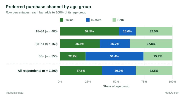
A 100% stacked bar chart such as Figure 1 is often the clearest way to show row percentages to a business audience. For tables with many categories, a mosaic display, in which the area of each tile is proportional to the cell count, shows both the marginal sizes and the departures from independence (Friendly, 1994). Whatever the format, avoid three-dimensional effects, unlabelled axes and inconsistent ordering, which make tables and charts easy to misread (Wainer, 1984).
Is the association real? The chi-square test
Differences in a sample table may arise by chance. The standard check is Pearson's chi-square test of independence. If age and channel were unrelated, the expected count in each cell would be its row total multiplied by its column total, divided by the grand total:
Eij = (row totali × column totalj) ÷ N
The test statistic adds up the squared gaps between observed counts O and expected counts E, scaled by the expected counts:
χ² = Σ (Oij − Eij)² ÷ Eij
with (rows − 1) × (columns − 1) degrees of freedom (Pearson, 1900). In Table 2, the expected count of online buyers aged 18–34 is 400 × 450 ÷ 1,200 = 150, against 210 observed. Across all nine cells, χ² ≈ 138.5 with 4 degrees of freedom, far beyond the 1% critical value of 13.3, so the hypothesis that channel preference is unrelated to age is clearly rejected in this illustrative example.
Small expected counts
The chi-square distribution is only an approximation, and it can be poor when expected counts are small. Cochran (1954) proposed the widely quoted guideline that no expected count should be below 1 and no more than about 20% should be below 5. For 2 × 2 tables, Yates (1934) introduced a continuity correction, but later work showed it is usually too conservative. In an extensive comparison, Campbell (2007) recommended a slightly modified "N − 1" chi-square test when every expected count is at least 1, and the Fisher–Irwin exact test otherwise. In practice, sparse tables are often better handled by merging thin categories in a way that still makes substantive sense.
How strong is the association?
A significant chi-square says only that an association is unlikely to be pure chance. With large survey samples even trivial differences become "significant", so a measure of strength is also needed. The most common is Cramér's V (Cramér, 1946):
V = √(χ² ÷ (N × (k − 1)))
where k is the smaller of the number of rows and columns. V runs from 0 (no association) to 1 (perfect association). For Table 2, V = √(138.5 ÷ (1,200 × 2)) ≈ 0.24, a moderate association. Goodman and Kruskal (1954) developed further measures, such as lambda, which tells how much knowing one variable improves the prediction of the other, and gamma, which suits two ordinal variables.
Where is the association? Adjusted residuals
A chi-square test covers the whole table. To see which cells drive the result, analysts use adjusted standardised residuals, which compare each observed count with its expected count and behave approximately like standard normal values when the variables are independent (Haberman, 1973). Values beyond about ±2 mark cells that differ noticeably from independence. In the example, the largest residuals are +10.4 for in-store buyers aged 55 and over, +7.6 for online buyers aged 18–34 and −8.0 for in-store buyers aged 18–34. Residuals in the "Both" column are much smaller, between −3.2 and +3.0, so the story is mainly a shift from online to in-store buying with age.
Survey data need survey methods
Standard chi-square formulas assume a simple random sample. Real surveys usually involve weights, stratification and clustering, which change the variance of estimated proportions. Rao and Scott (1981, 1984) showed that the ordinary Pearson statistic can then be badly misleading and proposed corrections that divide it by an estimate of the average design effect. Simulation work by Thomas and Rao (1987) compared such corrected tests and found that they kept error rates close to nominal levels where the uncorrected test did not. For example, if the design effect in the illustrative survey were around 1.5, a first-order correction would reduce χ² from 138.5 to about 92: still clearly significant here, but enough to remove borderline results in other tables. Modern survey software applies these corrections automatically when the design is declared (Heeringa et al., 2010; Lohr, 2021). Weighted percentages should be shown in the table, while the unweighted base should be reported beneath it.
Common mistakes
- Unclear bases. Percentages without a stated base, or bases that change silently from table to table, are the most frequent source of confusion.
- Percentaging the wrong way. Row and column percentages answer different questions; label which one is shown.
- Over-reading small cells. A subgroup of 30 respondents gives very imprecise percentages. Flag or suppress small bases.
- Testing everything. A full set of banner tables can contain hundreds of significance tests, and some will be "significant" by chance alone. Methods that control the false discovery rate limit the number of spurious findings (Benjamini & Hochberg, 1995).
- Ignoring a third variable. An association in a two-way table can weaken, vanish or reverse when the data are split by a third variable, a pattern known as Simpson's paradox (Simpson, 1951). The well-known analysis of graduate admissions at Berkeley found that an apparent bias against women in the pooled table largely disappeared within departments, because women applied more often to departments with low admission rates (Bickel et al., 1975).
- Treating association as causation. A strong cross-tabulation shows that two answers go together, not that one causes the other.
Key takeaways
Frequency tables and cross-tabulations are the backbone of survey reporting. State the base, choose the percentage direction that matches the question, and show a chart that makes the pattern easy to see. Use the chi-square test to judge whether an association is likely to be real, Cramér's V to judge its strength and adjusted residuals to locate it. For weighted or clustered samples, use design-adjusted tests, and always check whether a third variable could change the story.
References
Benjamini, Y., & Hochberg, Y. (1995). Controlling the false discovery rate: A practical and powerful approach to multiple testing. Journal of the Royal Statistical Society Series B: Statistical Methodology, 57(1), 289–300. https://doi.org/10.1111/j.2517-6161.1995.tb02031.x
Bickel, P. J., Hammel, E. A., & O'Connell, J. W. (1975). Sex bias in graduate admissions: Data from Berkeley. Science, 187(4175), 398–404. https://doi.org/10.1126/science.187.4175.398
Campbell, I. (2007). Chi-squared and Fisher–Irwin tests of two-by-two tables with small sample recommendations. Statistics in Medicine, 26(19), 3661–3675. https://doi.org/10.1002/sim.2832
Cochran, W. G. (1954). Some methods for strengthening the common χ² tests. Biometrics, 10(4), 417–451. https://doi.org/10.2307/3001616
Cramér, H. (1946). Mathematical methods of statistics. Princeton University Press. https://doi.org/10.1515/9781400883868
Fagerland, M. W., Lydersen, S., & Laake, P. (2017). Statistical analysis of contingency tables. Chapman and Hall/CRC. https://doi.org/10.1201/9781315374116
Friendly, M. (1994). Mosaic displays for multi-way contingency tables. Journal of the American Statistical Association, 89(425), 190–200. https://doi.org/10.1080/01621459.1994.10476460
Goodman, L. A., & Kruskal, W. H. (1954). Measures of association for cross classifications. Journal of the American Statistical Association, 49(268), 732–764. https://doi.org/10.1080/01621459.1954.10501231
Haberman, S. J. (1973). The analysis of residuals in cross-classified tables. Biometrics, 29(1), 205–220. https://doi.org/10.2307/2529686
Heeringa, S. G., West, B. T., & Berglund, P. A. (2010). Applied survey data analysis. Chapman and Hall/CRC. https://doi.org/10.1201/9781420080674
Lohr, S. L. (2021). Sampling: Design and analysis (3rd ed.). Chapman and Hall/CRC. https://doi.org/10.1201/9780429298899
Pearson, K. (1900). On the criterion that a given system of deviations from the probable in the case of a correlated system of variables is such that it can be reasonably supposed to have arisen from random sampling. The London, Edinburgh, and Dublin Philosophical Magazine and Journal of Science, 50(302), 157–175. https://doi.org/10.1080/14786440009463897
Rao, J. N. K., & Scott, A. J. (1981). The analysis of categorical data from complex sample surveys: Chi-squared tests for goodness of fit and independence in two-way tables. Journal of the American Statistical Association, 76(374), 221–230. https://doi.org/10.1080/01621459.1981.10477633
Rao, J. N. K., & Scott, A. J. (1984). On chi-squared tests for multiway contingency tables with cell proportions estimated from survey data. The Annals of Statistics, 12(1), 46–60. https://doi.org/10.1214/aos/1176346391
Simpson, E. H. (1951). The interpretation of interaction in contingency tables. Journal of the Royal Statistical Society Series B: Statistical Methodology, 13(2), 238–241. https://doi.org/10.1111/j.2517-6161.1951.tb00088.x
Thomas, D. R., & Rao, J. N. K. (1987). Small-sample comparisons of level and power for simple goodness-of-fit statistics under cluster sampling. Journal of the American Statistical Association, 82(398), 630–636. https://doi.org/10.1080/01621459.1987.10478476
Wainer, H. (1984). How to display data badly. The American Statistician, 38(2), 137–147. https://doi.org/10.1080/00031305.1984.10483186
Yates, F. (1934). Contingency tables involving small numbers and the χ² test. Journal of the Royal Statistical Society Series B: Statistical Methodology, 1(2), 217–235. https://doi.org/10.2307/2983604