
Statistics · Descriptive statistics
Weighted Means and Weighted Percentages
How weighted means and weighted percentages work, why surveys need them, and how to check that weighting has not cost more precision than it gained.
An ordinary average treats every observation as equally important. In many real datasets that assumption is false. Some respondents stand for more people than others, some stores sell more than others, and some survey groups were sampled at higher rates than others. A weighted mean corrects for this by letting each observation count in proportion to what it represents. Weighting is one of the most common steps in survey analysis, and one of the most commonly misunderstood.
The formula
For values x1 … xn with weights w1 … wn, the weighted mean is the sum of each value multiplied by its weight, divided by the sum of the weights:
x̄w = Σ wixi ÷ Σ wi
When every weight is 1, this reduces to the ordinary mean. A weighted percentage is the same calculation applied to a yes/no variable coded 1 and 0: it is the sum of the weights of the people who said "yes", divided by the sum of all weights.
Why surveys need weights
Survey samples rarely match the population exactly. Some designs deliberately oversample small groups so that they can be analysed separately; others end up unbalanced because some kinds of people are easier to reach or more willing to respond. In probability sampling, the starting weight for each respondent is the inverse of their probability of selection, so a person sampled with a 1-in-500 chance stands for 500 people (Horvitz & Thompson, 1952; Kish, 1965; Lohr, 2021). Analysts then usually adjust these base weights so that the weighted sample matches known population totals for age, sex, region or other characteristics, a step known as post-stratification, raking or calibration (Deville & Särndal, 1992; Kalton & Flores-Cervantes, 2003).
A worked example
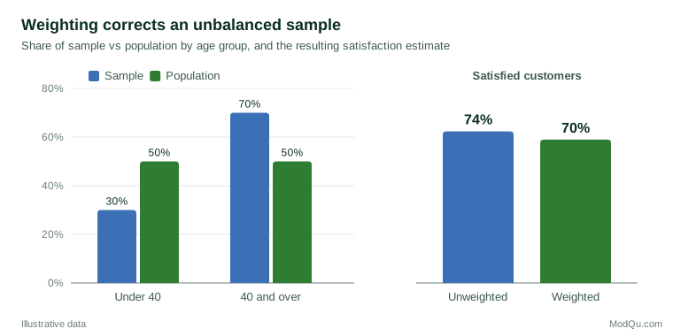
Suppose a company surveys 1,000 customers. Its records show that customers are split evenly between people under 40 and people aged 40 and over, but the sample contains 300 younger and 700 older respondents. Sixty percent of the younger group and 80% of the older group say they are satisfied.
The unweighted result is 740 satisfied out of 1,000, or 74%. That figure overstates satisfaction because the more satisfied older group is over-represented. To correct it, each younger respondent receives a weight of 0.50 ÷ 0.30 ≈ 1.67 and each older respondent a weight of 0.50 ÷ 0.70 ≈ 0.71. The weighted percentage is then (0.5 × 60%) + (0.5 × 80%) = 70%, a four-point difference that could change a business decision.
The cost of weighting
Weighting reduces bias, but it is not free. Unequal weights increase the variance of estimates, which means wider confidence intervals. Kish (1992) gave a widely used approximation for this loss, the effective sample size:
neff = (Σ wi)² ÷ Σ wi²
In the example above, the 1,000 interviews carry about as much precision as 840 equally weighted ones, a design effect of roughly 1.19. That is a reasonable price for removing a four-point bias. Very large or very uneven weights, however, can make a few respondents dominate the results. Practitioners therefore often trim extreme weights or collapse small weighting groups, accepting a little bias in exchange for a large gain in stability (Kalton & Flores-Cervantes, 2003).
Common mistakes
- Averaging percentages without weights. The mean of 60% and 80% is 70% only when the two groups are the same size in the population. For unequal groups, each percentage must be weighted by its group's population share.
- Reporting the weighted sum as the sample size. The number of interviews and the precision of the estimate are different things. Report both the unweighted count and, where relevant, the effective sample size.
- Using ordinary formulas for standard errors. Standard software formulas assume equal weights and simple random sampling. Weighted data needs survey-aware variance estimation (Lohr, 2021).
- Weighting on variables unrelated to the outcome. Weighting only removes bias when the weighting variables are related both to who responds and to the answers being measured. Otherwise it adds variance without reducing bias.
Key takeaways
A weighted mean lets each observation count for what it represents. In surveys, weights correct for unequal selection chances and for samples that do not match the population. Weighting usually reduces bias but increases variance, so good practice is to report weighted estimates together with the unweighted sample size and an honest measure of precision.
References
Deville, J.-C., & Särndal, C.-E. (1992). Calibration estimators in survey sampling. Journal of the American Statistical Association, 87(418), 376–382. https://doi.org/10.1080/01621459.1992.10475217
Horvitz, D. G., & Thompson, D. J. (1952). A generalization of sampling without replacement from a finite universe. Journal of the American Statistical Association, 47(260), 663–685. https://doi.org/10.1080/01621459.1952.10483446
Kalton, G., & Flores-Cervantes, I. (2003). Weighting methods. Journal of Official Statistics, 19(2), 81–98.
Kish, L. (1965). Survey sampling. Wiley.
Kish, L. (1992). Weighting for unequal Pi. Journal of Official Statistics, 8(2), 183–200.
Lohr, S. L. (2021). Sampling: Design and analysis (3rd ed.). CRC Press. https://doi.org/10.1201/9780429298899