
Statistics · Descriptive statistics
Measures of Central Tendency: Mean, Median and Mode
What the mean, median and mode each measure, how skewed data and outliers pull them apart, and how to choose the right "average" for survey and business reporting.
Almost every report contains an average: a single number that stands for a whole set of values. Statisticians call such a number a measure of central tendency, and there are three classic ones: the mean, the median and the mode. Each answers a slightly different question about where the "middle" of the data lies. When data are skewed or contain extreme values, they can tell very different stories, and the wrong choice can mislead without any error in the arithmetic.
The mean
The arithmetic mean is the sum of the values divided by their number. For values x1 … xn:
x̄ = Σ xi ÷ n
The mean uses every observation and is the basis of most statistical inference. It is the value that minimises the sum of squared deviations, and the total of a variable is simply the mean multiplied by the number of cases, which makes it the natural choice whenever totals matter, such as revenue or volume forecasts. When observations represent different numbers of people, as in a weighted survey, the weighted mean lets each value count in proportion to what it represents (Lohr, 2021).
The mean's weakness is its sensitivity to extreme values. A single very large observation can move it a long way. In the language of robust statistics, the mean has a breakdown point of zero: one sufficiently wild value can push it anywhere (Hampel, 1974; Huber, 1964).
The median
The median is the middle value when the observations are sorted. With an odd number of values it is the one in the centre; with an even number it is usually taken as the average of the two central values. Half of the observations lie at or below the median and half at or above it. Where the mean minimises squared deviations, the median minimises the sum of absolute deviations.
The median is robust: it is barely affected by a few extreme values, and up to half of the data would have to be corrupted before it could be driven to an arbitrary value. This is why income and house prices are usually reported as medians. Using the middle value to resist extreme opinions has a long history. Galton (1907) analysed nearly 800 guesses of an ox's weight at a country fair and argued for the median as the fair "vote" of the crowd, because no single eccentric guess could sway it; the idea had been used informally well before that (Bakker & Gravemeijer, 2006).
The mode
The mode is the most frequent value, the term itself having been introduced by Pearson (1895). It is the only one of the three measures that can be used for nominal data, such as favourite brand, region or preferred channel, where values cannot be added or ranked. For continuous data the mode refers to the peak of the distribution, and some distributions have two or more peaks (bimodal or multimodal), which is often a sign that two different groups have been combined.
The mode can be unstable: in small samples one extra response may change it, and continuous data may need grouping into bins before any value repeats.
A worked example
Suppose a hypothetical retailer records the spending of nine customers in one month, in dollars:
| Customer | 1 | 2 | 3 | 4 | 5 | 6 | 7 | 8 | 9 |
|---|---|---|---|---|---|---|---|---|---|
| Spend ($) | 40 | 55 | 60 | 60 | 70 | 85 | 90 | 110 | 930 |
The total is $1,500, so the mean is $1,500 ÷ 9 ≈ $166.67. The median is the fifth sorted value, $70. The mode is $60, the only value that appears twice.
The mean is more than twice the median, and only one of the nine customers actually spent more than the mean. The cause is the single $930 customer. Remove that customer and the mean falls to $71.25, while the median moves only from $70 to $65. To forecast total revenue, the mean is the relevant figure, because totals depend on every dollar spent. To describe what a typical customer spends, the median is far more representative.
Skewness pulls the measures apart
Many business variables are right-skewed: most values are modest, but a long tail of large values stretches to the right. Income, purchase amounts, time on site, claim sizes and company revenues all tend to look like this, and many follow distributions close to the log-normal (Limpert et al., 2001). Truly symmetric, bell-shaped data are less common in practice than textbooks suggest; Micceri (1989) examined 440 large-sample distributions of achievement and psychometric measures and found that none passed every test of normality.
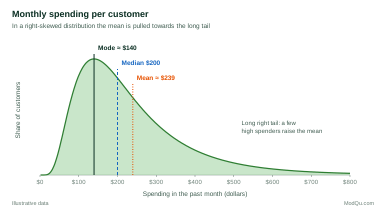
In a right-skewed distribution like Figure 1 the usual ordering is mode, then median, then mean. A common textbook rule says this ordering always holds, and that the mean lies on the side of the longer tail. Research by von Hippel (2005) showed that the rule fails surprisingly often, especially for discrete data and for distributions in which one tail is long but the other is heavy. The comparison of mean and median is therefore a useful warning sign rather than a formal test of skewness; for that, a skewness coefficient is better (Doane & Seward, 2011).
Choosing the right measure
The level of measurement sets the first limit on what is meaningful (Stevens, 1946):
| Level of measurement | Example | Mode | Median | Mean |
|---|---|---|---|---|
| Nominal | Preferred brand | Yes | No | No |
| Ordinal | Satisfaction (very poor to very good) | Yes | Yes | Debated |
| Interval or ratio | Spend, age, time | Yes | Yes | Yes |
Beyond that, the choice depends on the purpose and the shape of the data:
- Use the mean when totals or sums matter, when the data are roughly symmetric, or when the result feeds into further calculations such as regression or forecasting.
- Use the median to describe a typical case in skewed data, such as income, prices or durations, or when a few extreme values or data errors may be present.
- Use the mode for categorical answers, or to identify the most common response or price point.
- Report more than one when they differ noticeably. The gap between mean and median is itself informative.
Rating scales
Survey rating scales sit in the contested middle row of the table. Strictly, the points of a five-point agreement scale are ordered categories, and some authors argue that only the median and mode are appropriate (Jamieson, 2004). Others show that parametric methods based on means are robust enough for such data in most practical situations (Norman, 2010). A sensible compromise is to report the mean together with the full distribution or a "top-two box" percentage, so readers can see whether an average of 3.5 reflects broad agreement or a polarised split.
Robust alternatives
Between the mean and the median lie compromise measures. The trimmed mean discards a fixed percentage of the highest and lowest values (say 10% from each end) and averages the rest; the winsorised mean replaces those extreme values with the nearest remaining ones instead of dropping them. Both keep much of the mean's efficiency while greatly reducing sensitivity to outliers, and Wilcox and Keselman (2003) recommend them for comparing groups when data are skewed or heavy-tailed. Huber (1964) developed a more general family, M-estimators, that down-weights rather than discards extreme observations.
Common mistakes
- Calling any figure "the average" without saying which one. "Average salary" might be a mean or a median. State the measure.
- Deleting outliers to make the mean look sensible. Investigate extreme values first. They may be errors, or they may be the most commercially important customers. Robust measures, or outlier rules based on the median absolute deviation rather than the standard deviation, are usually safer than ad hoc deletion (Leys et al., 2013).
- Averaging averages. The mean of group means equals the overall mean only when the groups are the same size; otherwise each group mean must be weighted by its size.
- Ignoring survey weights. In weighted samples, the mean, median and mode should all be computed with the weights.
Key takeaways
The mean uses every value and is essential for totals, but it is easily pulled by extreme values. The median describes the typical case and resists outliers, which makes it the better choice for skewed data such as income and spending. The mode is the only option for categories and shows the most common answer. Good practice is to choose the measure that matches the question and the level of measurement, to look at the shape of the data first, and to report more than one measure when they disagree.
References
Bakker, A., & Gravemeijer, K. P. E. (2006). An historical phenomenology of mean and median. Educational Studies in Mathematics, 62(2), 149–168. https://doi.org/10.1007/s10649-006-7099-8
Doane, D. P., & Seward, L. E. (2011). Measuring skewness: A forgotten statistic? Journal of Statistics Education, 19(2). https://doi.org/10.1080/10691898.2011.11889611
Galton, F. (1907). Vox populi. Nature, 75(1949), 450–451. https://doi.org/10.1038/075450a0
Hampel, F. R. (1974). The influence curve and its role in robust estimation. Journal of the American Statistical Association, 69(346), 383–393. https://doi.org/10.1080/01621459.1974.10482962
Huber, P. J. (1964). Robust estimation of a location parameter. The Annals of Mathematical Statistics, 35(1), 73–101. https://doi.org/10.1214/aoms/1177703732
Jamieson, S. (2004). Likert scales: How to (ab)use them. Medical Education, 38(12), 1217–1218. https://doi.org/10.1111/j.1365-2929.2004.02012.x
Leys, C., Ley, C., Klein, O., Bernard, P., & Licata, L. (2013). Detecting outliers: Do not use standard deviation around the mean, use absolute deviation around the median. Journal of Experimental Social Psychology, 49(4), 764–766. https://doi.org/10.1016/j.jesp.2013.03.013
Limpert, E., Stahel, W. A., & Abbt, M. (2001). Log-normal distributions across the sciences: Keys and clues. BioScience, 51(5), 341–352. https://doi.org/10.1641/0006-3568(2001)051[0341:LNDATS]2.0.CO;2
Lohr, S. L. (2021). Sampling: Design and analysis (3rd ed.). CRC Press. https://doi.org/10.1201/9780429298899
Micceri, T. (1989). The unicorn, the normal curve, and other improbable creatures. Psychological Bulletin, 105(1), 156–166. https://doi.org/10.1037/0033-2909.105.1.156
Norman, G. (2010). Likert scales, levels of measurement and the "laws" of statistics. Advances in Health Sciences Education, 15(5), 625–632. https://doi.org/10.1007/s10459-010-9222-y
Pearson, K. (1895). Contributions to the mathematical theory of evolution. II. Skew variation in homogeneous material. Philosophical Transactions of the Royal Society of London (A), 186, 343–414. https://doi.org/10.1098/rsta.1895.0010
Stevens, S. S. (1946). On the theory of scales of measurement. Science, 103(2684), 677–680. https://doi.org/10.1126/science.103.2684.677
von Hippel, P. T. (2005). Mean, median, and skew: Correcting a textbook rule. Journal of Statistics Education, 13(2). https://doi.org/10.1080/10691898.2005.11910556
Wilcox, R. R., & Keselman, H. J. (2003). Modern robust data analysis methods: Measures of central tendency. Psychological Methods, 8(3), 254–274. https://doi.org/10.1037/1082-989X.8.3.254