
Statistics · Survey statistics
Significance Testing in Cross-Tabulated Survey Results
How the significance letters and arrows in survey banner tables are produced, why weighting and multiple comparisons change them, and how to report differences between subgroups honestly.
The standard output of a commercial survey is the banner table: a cross-tabulation with the survey questions down the side and subgroups such as region, age, gender or customer type across the top. Most banner tables also carry small letters, arrows or coloured cells that flag differences between columns as "statistically significant". Readers rely heavily on those flags. A brand manager scanning forty pages of tables will usually look for the letters first and the numbers second.
This article explains what those flags mean and how they are calculated, and shows why the default settings of tabulation software often produce more "significant" differences than the data support. It covers the overall test of a table, pairwise column tests, the effect of weighting and sample design, the problem of multiple comparisons, and practical rules for reporting. A companion article covers the chi-square test itself in more depth; here the focus is on the many tests that a single banner table contains.
Two questions a cross-tab can answer
A significance test in a cross-tabulation can address two quite different questions.
The first is whether a row variable and a column variable are associated at all. Is brand awareness related to region? The usual tool is Pearson's chi-square test of independence (Pearson, 1900), which compares the observed counts in every cell with the counts expected if the two variables were unrelated. It produces one p-value for the whole table.
The second is whether two particular columns differ on a particular row. Is awareness in the West higher than in Atlantic Canada? This is a comparison of two proportions, usually made with a z-test, and a banner table may contain hundreds of them. The significance letters in a banner table almost always come from this second kind of test.
The two questions should be kept apart. An overall test can be significant even when no single pair of columns differs reliably, and a pair of columns can differ even when the overall test is not significant, especially in large tables where one real difference is diluted by many cells with none.
How column letters are produced
In a typical banner, each column is given a letter. Under each percentage, the table shows the letters of the columns that are significantly lower. For two columns i and j with proportions pi and pj and bases ni and nj, the classic test statistic is:
z = (pi − pj) ÷ √[p̄(1 − p̄)(1/ni + 1/nj)]
where p̄ is the pooled proportion of the two columns combined. If |z| exceeds 1.96, the difference is flagged at the 5% level. The test assumes the two columns are independent samples, that the bases are the actual numbers of respondents, and that respondents were selected by simple random sampling. In real surveys, all three assumptions are often false.
A worked example
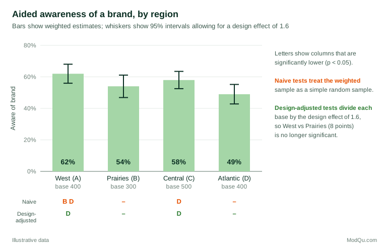
Consider a hypothetical brand tracker of 1,600 respondents, weighted to population targets, with four regional columns: West (A, base 400), Prairies (B, 300), Central (C, 500) and Atlantic (D, 400). Aided awareness of the brand is 62%, 54%, 58% and 49% respectively.
Treating the data as a simple random sample, the pairwise tests give three significant differences: West is higher than Prairies (z = 2.13, p = 0.034) and higher than Atlantic (z = 3.70, p < 0.001), and Central is higher than Atlantic (z = 2.69, p = 0.007). The table would show "B D" under West and "D" under Central.
Weighting and design effects
Almost every commercial survey is weighted, and many use clustered or stratified samples. Both change the precision of estimates. The usual summary is the design effect: the ratio of the actual variance of an estimate to the variance it would have under simple random sampling of the same size (Lohr, 2021). Weighting alone typically produces design effects above 1, because unequal weights make some respondents count more than others. A widely used approximation for the design effect due to weighting is 1 plus the squared coefficient of variation of the weights (Valliant et al., 2018).
Dividing the base by the design effect gives the effective sample size, the number of simple random sample respondents that would provide the same precision. In the example, suppose the design effect is 1.6. Then the West column's 400 respondents carry the information of only 250, and the 95% margin of error around its 62% widens from about ±4.8 to about ±6.0 percentage points.
Repeating the pairwise tests with effective bases changes the picture (Figure 1). West versus Atlantic (p = 0.003) and Central versus Atlantic (p = 0.033) remain significant, but West versus Prairies does not (z = 1.68, p = 0.093). One of the three letters disappears. That is a typical result: tabulation software that tests weighted percentages against unweighted or, worse, weighted bases as though they came from a simple random sample overstates significance, sometimes substantially.
The same applies to the overall chi-square test. Rao and Scott (1981, 1984) showed that, under complex sampling, the ordinary Pearson statistic no longer follows a chi-square distribution, and they proposed corrected statistics that, in the simplest version, divide it by an estimate of the average design effect. Thomas and Rao (1987) found in simulations that such corrections kept the error rate close to the nominal level where the uncorrected test did not. In the example, the naive chi-square for awareness by region is 15.1 on 3 degrees of freedom (p = 0.002); dividing by 1.6 gives 9.4 (p = 0.024). The conclusion holds here, but in other tables the correction will turn a borderline "significant" result into a non-significant one. Survey analysis software applies these corrections automatically once the weights, strata and clusters are declared (Heeringa et al., 2010; Lumley, 2010).
Two practical consequences follow. First, a banner table should state whether its tests allow for weighting and design. Second, testing should use effective bases, not weighted counts. Weighted counts scaled to a population of millions make every difference look significant; weighted counts scaled to the sample size still ignore the loss of precision from weighting.
Multiple comparisons
A banner with four columns has six possible pairs. A ten-row question then involves 60 pairwise tests, and a full report with 40 questions and two banners can involve thousands. Each test run at the 5% level has a 5% chance of flagging a difference when there is none. Across many tests these chances accumulate. If all the null hypotheses were true and the tests were independent, the chance of at least one false positive would be 1 − 0.95k for k tests: 26% for six tests, 64% for 20 and 95% for 60 (Figure 2). In a typical report, the expected number of false alarms is simply 5% of the number of tests: about three among 60, and about 50 among 1,000.
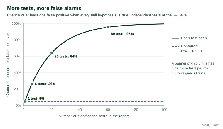
Tests within a banner are not fully independent, so the exact figures differ, but the lesson does not. A report that flags every p below 0.05 will contain some false findings, and readers cannot tell which ones they are. Simmons et al. (2011) showed how flexibility in choosing which comparisons to report can make almost any pattern look significant. A banner table invites exactly this kind of selective reading.
There are three main responses.
- Control the familywise error rate. The Bonferroni method tests each comparison at α ÷ k, where k is the number of comparisons in a family (Dunn, 1961). With six pairs, each is tested at 0.05 ÷ 6 ≈ 0.008. In the example, only West versus Atlantic survives. The method is simple and safe, but it is conservative when k is large and loses power to detect real differences.
- Control the false discovery rate. Benjamini and Hochberg (1995) proposed controlling the expected proportion of flagged results that are false, rather than the chance of any false result. Their procedure sorts the p-values, compares the rth smallest with (r ÷ k) × α, and flags all results up to the largest that passes. It is far more powerful than Bonferroni when many tests are run and is well suited to screening large tables.
- Test a few planned comparisons. Decide before seeing the data which differences matter for the business question, and test those at the usual level. Treat everything else as exploratory.
What counts as a "family" is a judgement. A sensible default for banner tables is one family per question and banner, so that the six region pairs for one row form one family. Whatever the choice, the report should say what was done.
Other technical pitfalls in banner tables
Testing a column against the total
Many banners include a total column, and some software tests each subgroup against it. But the total contains the subgroup, so the two are not independent samples, and the standard two-sample test is wrong. In the example, West makes up a quarter of the total, which pulls the total (56%) towards West's 62%. The correct comparison is West against the rest of the sample (54%), or a test that allows for the overlap.
Overlapping columns
Banners often include columns that share respondents: "buyers of brand X" and "buyers of brand Y", or "under 35" and "students". Respondents who appear in both columns make the two percentages correlated, and an independent-samples test gives the wrong answer. Some tabulation packages offer overlap-corrected tests; where they do not, such comparisons should not be flagged.
Multiple-response questions
On a "select all that apply" question, the percentages in a column add up to more than 100%. Comparing two rows within a column, such as whether more people chose "price" than "quality", involves the same respondents twice. Comparisons across columns for one row are fine, but comparisons between rows need methods for paired proportions.
Small bases and sparse tables
Approximate tests rely on reasonably large expected counts. Cochran (1954) suggested that the chi-square approximation is adequate when no expected count is below 1 and no more than 20% are below 5. For 2 × 2 tables, Campbell (2007) found that an "N − 1" version of the chi-square test performs well when all expected counts are at least 1, and recommended the Fisher–Irwin exact test otherwise. Yates' continuity correction (Yates, 1934) is often applied by default but tends to be overly conservative. For proportions near 0% or 100%, or in small columns, the simple Wald interval behaves poorly, and score-based intervals are better (Agresti & Coull, 1998). Fagerland et al. (2017) review recommended methods for all common table types. In practice, many research teams set a minimum base, such as 50 or 100 respondents, below which columns are shown but not tested.
Comparing waves of a tracker
Wave-on-wave changes in a tracker are tested in the same way as columns, provided the waves are independent samples. If some respondents take part in both waves, the samples overlap and the test should allow for the correlation, as with overlapping banner columns. Trackers also invite a subtle form of multiple testing: a team that checks every measure every month will see a "significant" movement somewhere almost every month. Looking for changes that persist over several waves, or smoothing with a rolling average, gives a steadier signal.
Significant is not the same as important
A significance letter says only that a difference is unlikely to be due to sampling variation alone, under the assumptions of the test. It says nothing about whether the difference is large enough to matter. The American Statistical Association's statement on p-values stresses that a p-value does not measure the size of an effect or the importance of a result (Wasserstein & Lazar, 2016), and Greenland et al. (2016) catalogue the most common misreadings.
In large samples, trivial differences become significant. A tracker of 20,000 respondents will flag a two-point difference in awareness between regions, which may have no commercial meaning. In small samples, important differences may not reach significance. Three habits help:
- Report effect sizes and intervals. For a whole table, Cramér's V (Cramér, 1946) scales the chi-square statistic to lie between 0 and 1. In the example, V ≈ 0.10, which is small by Cohen's (1988) conventions for this kind of measure. For a pair of columns, report the difference in percentage points with its confidence interval.
- Do not read "no letter" as "no difference". A non-significant result may reflect a small base rather than equality. Absence of evidence is not evidence of absence (Altman & Bland, 1995).
- Do not compare significance levels. Gelman and Stern (2006) point out that the difference between "significant" and "not significant" is not itself statistically significant. In the example, Central differs significantly from Atlantic and Prairies does not, yet Central and Prairies do not differ significantly from each other (p = 0.38 with design adjustment). Concluding that Central "behaves differently" from Prairies on this basis would be a mistake.
Overlapping confidence intervals are a related trap. Two 95% intervals can overlap even when the difference between the estimates is significant, because the standard error of a difference is smaller than the sum of the two standard errors. Schenker and Gentleman (2001) show that checking for overlap is a conservative test, so it misses some real differences. Under simple random sampling, the West and Prairies intervals overlap even though the naive test flags them as different.
Practical guidance for survey teams
- Declare the design. Run tests in software that knows the weights, strata and clusters, or at least use effective bases.
- Start with the question. Use an overall test of the table to decide whether there is anything to explain, and then use pairwise tests to locate it.
- Limit and adjust comparisons. Define families of tests, apply a Bonferroni or false discovery rate adjustment, and say which method was used in a footnote to every table.
- Set minimum bases. Do not test columns with very small effective bases, and flag them clearly.
- Avoid invalid comparisons. Do not test columns against a total that contains them, or overlapping columns, without a correction.
- Lead with size, not stars. Report percentage-point differences and intervals, and discuss whether they matter for the decision at hand.
Key takeaways
Significance letters in banner tables come from many pairwise tests, each of which assumes independent simple random samples. Weighting and complex designs reduce effective sample sizes, so naive tests overstate significance; design-based corrections such as the Rao–Scott adjustment and effective bases fix this. Running hundreds of tests guarantees false positives, which Bonferroni or false discovery rate methods can control. Comparisons with a total, overlapping columns, multiple-response rows and small bases each need special care. Finally, a significant difference is not necessarily an important one, and a non-significant one is not proof of equality. Clear reporting of differences, intervals and methods serves decision-makers better than a page of letters.
References
Agresti, A., & Coull, B. A. (1998). Approximate is better than "exact" for interval estimation of binomial proportions. The American Statistician, 52(2), 119–126. https://doi.org/10.1080/00031305.1998.10480550
Altman, D. G., & Bland, J. M. (1995). Absence of evidence is not evidence of absence. BMJ, 311(7003), 485. https://doi.org/10.1136/bmj.311.7003.485
Benjamini, Y., & Hochberg, Y. (1995). Controlling the false discovery rate: A practical and powerful approach to multiple testing. Journal of the Royal Statistical Society Series B: Statistical Methodology, 57(1), 289–300. https://doi.org/10.1111/j.2517-6161.1995.tb02031.x
Campbell, I. (2007). Chi-squared and Fisher–Irwin tests of two-by-two tables with small sample recommendations. Statistics in Medicine, 26(19), 3661–3675. https://doi.org/10.1002/sim.2832
Cochran, W. G. (1954). Some methods for strengthening the common χ² tests. Biometrics, 10(4), 417–451. https://doi.org/10.2307/3001616
Cohen, J. (1988). Statistical power analysis for the behavioral sciences (2nd ed.). Routledge. https://doi.org/10.4324/9780203771587
Cramér, H. (1946). Mathematical methods of statistics. Princeton University Press. https://doi.org/10.1515/9781400883868
Dunn, O. J. (1961). Multiple comparisons among means. Journal of the American Statistical Association, 56(293), 52–64. https://doi.org/10.1080/01621459.1961.10482090
Fagerland, M. W., Lydersen, S., & Laake, P. (2017). Statistical analysis of contingency tables. Chapman and Hall/CRC. https://doi.org/10.1201/9781315374116
Gelman, A., & Stern, H. S. (2006). The difference between "significant" and "not significant" is not itself statistically significant. The American Statistician, 60(4), 328–331. https://doi.org/10.1198/000313006X152649
Greenland, S., Senn, S. J., Rothman, K. J., Carlin, J. B., Poole, C., Goodman, S. N., & Altman, D. G. (2016). Statistical tests, P values, confidence intervals, and power: A guide to misinterpretations. European Journal of Epidemiology, 31(4), 337–350. https://doi.org/10.1007/s10654-016-0149-3
Heeringa, S. G., West, B. T., & Berglund, P. A. (2010). Applied survey data analysis. Chapman and Hall/CRC. https://doi.org/10.1201/9781420080674
Lohr, S. L. (2021). Sampling: Design and analysis (3rd ed.). Chapman and Hall/CRC. https://doi.org/10.1201/9780429298899
Lumley, T. (2010). Complex surveys: A guide to analysis using R. Wiley. https://doi.org/10.1002/9780470580066
Pearson, K. (1900). On the criterion that a given system of deviations from the probable in the case of a correlated system of variables is such that it can be reasonably supposed to have arisen from random sampling. The London, Edinburgh, and Dublin Philosophical Magazine and Journal of Science, 50(302), 157–175. https://doi.org/10.1080/14786440009463897
Rao, J. N. K., & Scott, A. J. (1981). The analysis of categorical data from complex sample surveys: Chi-squared tests for goodness of fit and independence in two-way tables. Journal of the American Statistical Association, 76(374), 221–230. https://doi.org/10.1080/01621459.1981.10477633
Rao, J. N. K., & Scott, A. J. (1984). On chi-squared tests for multiway contingency tables with cell proportions estimated from survey data. The Annals of Statistics, 12(1), 46–60. https://doi.org/10.1214/aos/1176346391
Schenker, N., & Gentleman, J. F. (2001). On judging the significance of differences by examining the overlap between confidence intervals. The American Statistician, 55(3), 182–186. https://doi.org/10.1198/000313001317097960
Simmons, J. P., Nelson, L. D., & Simonsohn, U. (2011). False-positive psychology: Undisclosed flexibility in data collection and analysis allows presenting anything as significant. Psychological Science, 22(11), 1359–1366. https://doi.org/10.1177/0956797611417632
Thomas, D. R., & Rao, J. N. K. (1987). Small-sample comparisons of level and power for simple goodness-of-fit statistics under cluster sampling. Journal of the American Statistical Association, 82(398), 630–636. https://doi.org/10.1080/01621459.1987.10478476
Valliant, R., Dever, J. A., & Kreuter, F. (2018). Practical tools for designing and weighting survey samples (2nd ed.). Springer. https://doi.org/10.1007/978-3-319-93632-1
Wasserstein, R. L., & Lazar, N. A. (2016). The ASA statement on p-values: Context, process, and purpose. The American Statistician, 70(2), 129–133. https://doi.org/10.1080/00031305.2016.1154108
Yates, F. (1934). Contingency tables involving small numbers and the χ² test. Journal of the Royal Statistical Society Series B: Statistical Methodology, 1(2), 217–235. https://doi.org/10.2307/2983604