
Statistics · Tests and models
Principal Component Analysis and Dimension Reduction
How principal component analysis condenses many correlated survey questions into a few summary dimensions, how to decide how many to keep, and where the method helps or misleads.
Customer surveys often ask a dozen or more rating questions that overlap: people who rate a store's prices highly also tend to rate its promotions and value for money highly. Analysing each question separately produces long, repetitive tables and unstable models. Principal component analysis (PCA) replaces a set of correlated variables with a smaller set of uncorrelated summary variables, called components, that keep as much of the original information as possible. The idea goes back to Pearson (1901), who sought the lines and planes that best fit a cloud of points, and Hotelling (1933), who developed it as a method for analysing many related test scores.
How PCA works
Each principal component is a weighted sum of the original variables. The first component is the weighted sum with the largest possible variance; the second has the largest variance among weighted sums uncorrelated with the first; and so on, until there are as many components as variables:
PC1 = a11z1 + a12z2 + … + a1pzp
Here z1 to zp are the original variables, usually standardised, and the weights a come from the eigenvectors of their correlation (or covariance) matrix. The variance of each component is the corresponding eigenvalue. Because standardised variables each have variance 1, the eigenvalues of a correlation matrix add up to the number of variables, so an eigenvalue divided by that number gives the share of total variance a component explains (Jolliffe, 2002).
Geometrically, PCA rotates the axes of the data so that the first axis points along the direction of greatest spread. Keeping only the first few components gives the best possible low-dimensional approximation of the data in the least-squares sense, a result formalised by Eckart and Young (1936). Jolliffe and Cadima (2016) and Abdi and Williams (2010) give accessible modern reviews.
Correlation or covariance?
PCA on the covariance matrix lets variables with larger variances dominate. If items are measured in different units, such as spending in dollars and satisfaction on a 0 to 10 scale, the analysis must use the correlation matrix, which is the same as standardising every variable first. When all items share one rating scale, either choice is defensible, but the correlation matrix is the usual default in survey work (Jolliffe, 2002).
A worked example
Suppose a hypothetical grocery chain asks 600 shoppers to rate ten aspects of its stores. The numbers below come from simulated, illustrative data. PCA on the correlation matrix gives the eigenvalues in Figure 1.
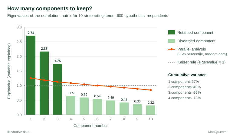
Three components have eigenvalues well above the rest and together explain 66% of the total variance; the fourth adds only 6.5 points. To make the components easier to interpret, the three are rotated with the varimax method (Kaiser, 1958), which redistributes the explained variance so that each item loads strongly on as few components as possible. The loadings, the correlations between items and components, are:
| Item | Value | Products | Service and convenience |
|---|---|---|---|
| Low prices | 0.86 | −0.02 | −0.02 |
| Frequent promotions | 0.83 | −0.05 | 0.03 |
| Good value for money | 0.86 | 0.00 | −0.03 |
| Fresh produce | −0.04 | 0.86 | 0.10 |
| Product quality | −0.05 | 0.86 | 0.14 |
| Wide range | 0.03 | 0.82 | −0.02 |
| Friendly staff | 0.03 | 0.15 | 0.75 |
| Short checkout queues | −0.04 | 0.03 | 0.75 |
| Easy parking | 0.01 | 0.03 | 0.72 |
| Clean, tidy store | −0.04 | 0.15 | 0.74 |
Ten ratings can now be summarised by three scores (value, products, and service and convenience) that can be tracked over time, compared across stores, or used as predictors of loyalty without the instability caused by highly correlated inputs. The names are the analyst's interpretation of the loading pattern; PCA itself supplies only numbers. The final column of a full output would also show each item's communality, the share of its variance captured by the retained components. Here communalities range from about 0.52 for easy parking to 0.76 for fresh produce and product quality, so every item is reasonably well represented.
Using component scores
Once the components are chosen, each respondent receives a score on each one, calculated from their standardised answers and the component weights. These scores have a mean of zero, so a store whose shoppers average +0.4 on the value component is rated better on value than the typical store in the sample. Scores can be fed into later analyses, such as a regression of loyalty on the three components, or compared between customer groups and survey waves.
Two practical cautions apply. First, exact component scores use every item, including those with small loadings, so many analysts prefer simple summated scales: the average of the items that load strongly on each component. These are easier to explain and more stable across samples, although they are no longer perfectly uncorrelated. Second, if the weights are re-estimated in every wave of a tracking study, the meaning of a score can drift. Fixing the weights from a reference wave keeps the scores comparable over time.
How many components to keep
Choosing the number of components is the most important decision in PCA. Several rules are in common use.
- The Kaiser rule keeps components with eigenvalues above 1, that is, those explaining more variance than a single original variable (Kaiser, 1960). It is simple but tends to keep too many components when there are many variables.
- The scree test looks for the point where the plotted eigenvalues level off into a gentle slope of "scree" (Cattell, 1966). It is useful but subjective.
- Parallel analysis compares each observed eigenvalue with the eigenvalues obtained from random data of the same size and keeps components that beat chance (Horn, 1965). In Figure 1, only the first three components exceed the 95th percentile of the random eigenvalues.
- Cumulative variance targets, such as 70% or 80%, are sometimes used but have no theoretical basis.
In an influential simulation, Zwick and Velicer (1986) found that parallel analysis was among the most accurate methods, while the Kaiser rule often overestimated the number of components. Parallel analysis is a sound default, ideally checked against the scree plot and the interpretability of the resulting components.
PCA is not factor analysis
PCA is often confused with factor analysis, and many software packages present them in the same menu. PCA is a data reduction technique: it summarises the total variance of the observed variables, including measurement error. Factor analysis is a measurement model: it assumes that a small number of unobserved factors cause the correlations among items, and it models only the shared variance. Velicer and Jackson (1990) argue that the two often give similar results in practice, especially with many variables and strong loadings. However, Fabrigar et al. (1999) recommend factor analysis when the goal is to identify latent constructs, such as attitudes or brand perceptions, and to build measurement scales. PCA is the better choice when the goal is simply to summarise or compress data.
Practical uses in business and survey data
- Summarising batteries of rating questions into a few stable scores for reporting and tracking.
- Reducing collinearity before regression or driver analysis, where many correlated predictors would otherwise produce erratic coefficients.
- Building composite indicators. The OECD handbook on composite indicators describes PCA as one way to explore the structure of indicator sets and to derive weights, while cautioning that statistical weights may not reflect the importance users attach to each indicator (Organisation for Economic Co-operation and Development [OECD] et al., 2008).
- Mapping brands or products on two or three dimensions, as in perceptual maps.
- Preparing inputs for segmentation, with caution. Dolnicar and Grün (2008) showed that clustering on component scores can obscure segments that clustering on the original items would find.
Limitations and common mistakes
- Over-reading component names. Labels summarise a loading pattern; they do not prove that a construct exists.
- Ignoring outliers. Because PCA is based on variances and correlations, a few extreme respondents can tilt the components. Robust versions such as ROBPCA reduce this sensitivity (Hubert et al., 2005).
- Assuming linearity. PCA captures linear relationships only. Curved or clustered structure may be missed.
- Treating rating scales as precise. PCA on short ordinal scales is common and usually workable, but very skewed items or items with few categories can distort correlations.
- Hard-to-read components. With many variables, every component may load a little on everything. Rotation helps, and sparse PCA, which forces many weights to exactly zero, is an alternative designed for interpretability (Zou et al., 2006).
- Forgetting the scale. Running PCA on unstandardised variables measured in different units mainly reflects which units happen to be largest.
- Trusting small samples. Loadings estimated from small samples are unstable. Splitting the sample in half and comparing the two solutions is a quick check that the structure is not an accident of the data.
- Applying the same weights everywhere without checking. Components derived in one sample or market may not hold in another, so the structure should be checked again in new data.
Key takeaways
PCA turns many correlated variables into a few uncorrelated components that keep most of the information. It is a fast, transparent way to summarise rating batteries, reduce collinearity and build indices. Use the correlation matrix when units differ, decide how many components to keep with parallel analysis rather than the eigenvalue-above-1 rule alone, rotate when interpretation matters, and remember that PCA summarises data rather than measuring latent constructs. Check outliers, report the variance explained, and treat component names as interpretations, not facts.
References
Abdi, H., & Williams, L. J. (2010). Principal component analysis. WIREs Computational Statistics, 2(4), 433–459. https://doi.org/10.1002/wics.101
Cattell, R. B. (1966). The scree test for the number of factors. Multivariate Behavioral Research, 1(2), 245–276. https://doi.org/10.1207/s15327906mbr0102_10
Dolnicar, S., & Grün, B. (2008). Challenging "factor–cluster segmentation". Journal of Travel Research, 47(1), 63–71. https://doi.org/10.1177/0047287508318910
Eckart, C., & Young, G. (1936). The approximation of one matrix by another of lower rank. Psychometrika, 1(3), 211–218. https://doi.org/10.1007/BF02288367
Fabrigar, L. R., Wegener, D. T., MacCallum, R. C., & Strahan, E. J. (1999). Evaluating the use of exploratory factor analysis in psychological research. Psychological Methods, 4(3), 272–299. https://doi.org/10.1037/1082-989X.4.3.272
Horn, J. L. (1965). A rationale and test for the number of factors in factor analysis. Psychometrika, 30(2), 179–185. https://doi.org/10.1007/BF02289447
Hotelling, H. (1933). Analysis of a complex of statistical variables into principal components. Journal of Educational Psychology, 24(6), 417–441. https://doi.org/10.1037/h0071325
Hubert, M., Rousseeuw, P. J., & Vanden Branden, K. (2005). ROBPCA: A new approach to robust principal component analysis. Technometrics, 47(1), 64–79. https://doi.org/10.1198/004017004000000563
Jolliffe, I. T. (2002). Principal component analysis (2nd ed.). Springer. https://doi.org/10.1007/b98835
Jolliffe, I. T., & Cadima, J. (2016). Principal component analysis: A review and recent developments. Philosophical Transactions of the Royal Society A: Mathematical, Physical and Engineering Sciences, 374(2065), 20150202. https://doi.org/10.1098/rsta.2015.0202
Kaiser, H. F. (1958). The varimax criterion for analytic rotation in factor analysis. Psychometrika, 23(3), 187–200. https://doi.org/10.1007/BF02289233
Kaiser, H. F. (1960). The application of electronic computers to factor analysis. Educational and Psychological Measurement, 20(1), 141–151. https://doi.org/10.1177/001316446002000116
Organisation for Economic Co-operation and Development, European Union, & Joint Research Centre. (2008). Handbook on constructing composite indicators: Methodology and user guide. OECD Publishing. https://doi.org/10.1787/9789264043466-en
Pearson, K. (1901). LIII. On lines and planes of closest fit to systems of points in space. The London, Edinburgh, and Dublin Philosophical Magazine and Journal of Science, 2(11), 559–572. https://doi.org/10.1080/14786440109462720
Velicer, W. F., & Jackson, D. N. (1990). Component analysis versus common factor analysis: Some issues in selecting an appropriate procedure. Multivariate Behavioral Research, 25(1), 1–28. https://doi.org/10.1207/s15327906mbr2501_1
Zou, H., Hastie, T., & Tibshirani, R. (2006). Sparse principal component analysis. Journal of Computational and Graphical Statistics, 15(2), 265–286. https://doi.org/10.1198/106186006X113430
Zwick, W. R., & Velicer, W. F. (1986). Comparison of five rules for determining the number of components to retain. Psychological Bulletin, 99(3), 432–442. https://doi.org/10.1037/0033-2909.99.3.432