
Statistics · Inference
Power Analysis for Planning Studies
Power analysis tells you how many respondents a survey or experiment needs before fieldwork begins. This guide explains the inputs, works through a survey example and covers the most common planning mistakes.
How many respondents do we need? It is one of the first questions asked about any survey or experiment. Too small a sample risks a study that cannot answer its own question; too large a sample wastes budget and respondents' time. Power analysis is the standard way to set a sample size in advance so that a planned comparison has a good chance of detecting an effect that matters (Cohen, 1988).
What power analysis does
Statistical power is the probability that a test will return a significant result when a real effect of a specified size exists. Power analysis links four quantities, so that fixing any three determines the fourth:
- Effect size: the smallest difference or relationship the study should be able to detect.
- Significance level (α): the accepted risk of a Type I error, usually 5%.
- Power (1 − β): the desired chance of detecting the effect, usually 80% or 90%.
- Sample size: the number of respondents or units, usually the quantity being solved for.
Done before data collection, power analysis is a planning tool. It answers "how many do we need?" or, when the budget is fixed, "what is the smallest effect this study can reliably detect?"
The basic calculation
For comparing two group means with equal group sizes, a widely used normal approximation gives the sample size per group as:
n = 2(z1−α/2 + z1−β)2 σ2 ÷ Δ2
Here σ is the standard deviation of the outcome, Δ is the smallest difference worth detecting, and the z values come from the standard normal distribution (1.96 for a two-sided α of 5%, 0.84 for 80% power). With these conventional values the formula simplifies to about 16σ² ÷ Δ² per group, a rule of thumb that is also used for online controlled experiments (Kohavi et al., 2020).
The ratio Δ ÷ σ is the standardised effect size, often called Cohen's d. Cohen (1992) suggested 0.2, 0.5 and 0.8 as rough benchmarks for small, medium and large effects. Figure 1 shows how strongly the required sample depends on it: because n depends on the square of the effect size, halving the effect roughly quadruples the sample needed.
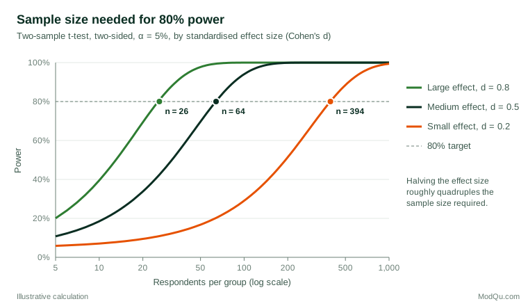
For proportions, regression coefficients, correlations or more complex models the formulas differ, but the logic is the same. Free software such as G*Power covers most standard tests (Faul et al., 2007).
A worked survey example
A hypothetical retailer wants to know whether satisfaction differs between customers who use its mobile app and those who do not. Satisfaction is measured on a 0 to 10 scale, and a previous wave of the tracker showed a standard deviation of about 2.0 points. The customer experience team agrees that a difference smaller than 0.6 points would not change any decision, so 0.6 is the smallest effect of interest, giving d = 0.6 ÷ 2.0 = 0.3.
The planning steps are:
| Step | Calculation | Respondents per group |
|---|---|---|
| Base sample for 80% power, α = 5% | 2 × 2.80² × 2.0² ÷ 0.6² | 175 |
| Design effect from weighting (assumed 1.5) | 175 × 1.5 | 263 |
| Allow 10% of completes removed in quality checks | 263 ÷ 0.90 | 293 |
An exact t-test calculation gives 176 rather than 175 for the first step, so the approximation is close. If app users make up only 20% of customers and the sample is drawn at random from the customer base, about 293 ÷ 0.20 ≈ 1,465 completed interviews are needed in total to yield enough app users, unless that group is deliberately oversampled.
The design effect matters in survey work. Kish (1965) showed that clustering and unequal weights increase the variance of estimates relative to a simple random sample, which reduces the effective sample size. A power calculation that ignores the design will overstate the power of the real study.
Choosing the effect size
The effect size is the most important input and the hardest to choose. There are three common sources:
- The smallest effect of practical interest. The best anchor is the difference that would change a business decision, such as the lift in conversion that would pay for a new feature. Lakens (2022) recommends stating this explicitly as part of any sample size justification.
- Previous studies or pilot data. These help, but published or pilot effects are often inflated, especially when they came from small samples (Button et al., 2013). Planning on an inflated effect produces an underpowered study.
- Generic benchmarks. Cohen's small, medium and large values are a last resort. Lenth (2001) warns that these "canned" effect sizes often say little about a particular study's context and can make a power analysis look more rigorous than it is.
The standard deviation must also be estimated, ideally from earlier waves of the same survey or from similar data.
Planning for precision instead of significance
Many descriptive surveys do not test a hypothesis at all; they estimate a share or an average. In that case it is more natural to plan for precision, choosing the sample so that the confidence interval is narrow enough to be useful. For a proportion near 50%, a margin of error of ±3 percentage points at 95% confidence requires about 1,068 respondents under simple random sampling (1.96² × 0.25 ÷ 0.03²), before any design effect. Maxwell et al. (2008) describe this approach, often called accuracy in parameter estimation, as a valuable complement to power analysis.
Complex designs and simulation
When the analysis involves multilevel data, several outcomes, unequal allocation or survey weights, closed-form formulas may not exist. Monte Carlo simulation offers a flexible alternative: generate many artificial data sets under assumed effect sizes and design features, analyse each one exactly as the real data will be analysed, and count how often the effect is detected (Arnold et al., 2011). Simulation also makes the assumptions visible to stakeholders.
Common mistakes
- Calculating power after the study. "Observed power" computed from the effect found in the data is a direct function of the p-value and adds no information (Hoenig & Heisey, 2001). Use confidence intervals to interpret a completed study instead.
- Powering only the total sample. Subgroup comparisons, such as regions or age bands, have much less power than the overall result. Plan for the most important subgroup comparison, not the headline figure.
- Ignoring multiple comparisons. If several outcomes or segments will be tested, the adjusted α is stricter and the required sample larger.
- Forgetting nonresponse and exclusions. Sample size calculations refer to usable completes, not invitations.
- Treating 80% as a guarantee. A study planned for 80% power still misses a true effect one time in five. When missing an effect is costly, 90% power is a sensible target.
- Over-trusting significant results from small studies. Even when they are significant, underpowered studies tend to exaggerate effect sizes (Gelman & Carlin, 2014).
Key takeaways
Power analysis turns a vague question about sample size into an explicit plan. Start from the smallest effect that would matter to the business, use realistic estimates of variability, and adjust for the survey design, subgroup comparisons and data losses. Where hypothesis testing is not the goal, plan for the precision of estimates instead. Document the assumptions, because a sample size is only as good as the inputs behind it.
References
Arnold, B. F., Hogan, D. R., Colford, J. M., Jr., & Hubbard, A. E. (2011). Simulation methods to estimate design power: An overview for applied research. BMC Medical Research Methodology, 11, Article 94. https://doi.org/10.1186/1471-2288-11-94
Button, K. S., Ioannidis, J. P. A., Mokrysz, C., Nosek, B. A., Flint, J., Robinson, E. S. J., & Munafò, M. R. (2013). Power failure: Why small sample size undermines the reliability of neuroscience. Nature Reviews Neuroscience, 14(5), 365–376. https://doi.org/10.1038/nrn3475
Cohen, J. (1988). Statistical power analysis for the behavioral sciences (2nd ed.). Routledge. https://doi.org/10.4324/9780203771587
Cohen, J. (1992). A power primer. Psychological Bulletin, 112(1), 155–159. https://doi.org/10.1037/0033-2909.112.1.155
Faul, F., Erdfelder, E., Lang, A.-G., & Buchner, A. (2007). G*Power 3: A flexible statistical power analysis program for the social, behavioral, and biomedical sciences. Behavior Research Methods, 39(2), 175–191. https://doi.org/10.3758/BF03193146
Gelman, A., & Carlin, J. (2014). Beyond power calculations: Assessing Type S (sign) and Type M (magnitude) errors. Perspectives on Psychological Science, 9(6), 641–651. https://doi.org/10.1177/1745691614551642
Hoenig, J. M., & Heisey, D. M. (2001). The abuse of power: The pervasive fallacy of power calculations for data analysis. The American Statistician, 55(1), 19–24. https://doi.org/10.1198/000313001300339897
Kish, L. (1965). Survey sampling. John Wiley & Sons.
Kohavi, R., Tang, D., & Xu, Y. (2020). Trustworthy online controlled experiments: A practical guide to A/B testing. Cambridge University Press. https://doi.org/10.1017/9781108653985
Lakens, D. (2022). Sample size justification. Collabra: Psychology, 8(1), Article 33267. https://doi.org/10.1525/collabra.33267
Lenth, R. V. (2001). Some practical guidelines for effective sample size determination. The American Statistician, 55(3), 187–193. https://doi.org/10.1198/000313001317098149
Maxwell, S. E., Kelley, K., & Rausch, J. R. (2008). Sample size planning for statistical power and accuracy in parameter estimation. Annual Review of Psychology, 59, 537–563. https://doi.org/10.1146/annurev.psych.59.103006.093735