
Statistics · Inference
Effect Sizes: Reporting What Matters Beyond Significance
A p-value says whether a difference is distinguishable from noise, not how big it is. This article explains the main effect sizes, how to calculate and read them, and how to report them.
A significance test answers a narrow question: is the observed difference larger than chance alone would comfortably produce? It does not say whether the difference is large, small or commercially relevant. With a big enough sample, almost any difference becomes "significant". The quantity that tells decision-makers what they actually want to know is the effect size: a number that expresses how large a difference or relationship is.
Kelley and Preacher (2012) define an effect size as a quantitative reflection of the magnitude of some phenomenon, used to address a question of interest. That definition is deliberately broad. A difference of 4 percentage points in brand awareness, a correlation of 0.3 between satisfaction and spend, and an odds ratio of 1.5 for renewal are all effect sizes. Reporting them has been standard advice for decades (Wilkinson & the Task Force on Statistical Inference, 1999) and is now required by major style guides (American Psychological Association, 2020).
Two families of effect size
Most effect sizes fall into two families (Cohen, 1988; Fritz et al., 2012).
- Difference measures compare groups: the raw difference in means or proportions, the standardised mean difference (Cohen's d or Hedges' g), the risk ratio and the odds ratio.
- Association measures describe how strongly variables move together: the correlation coefficient r, R² in regression, and eta-squared (η²) in analysis of variance, which give the share of variance explained.
Raw (unstandardised) effects
The simplest effect size is often the best. If a new checkout page lifts conversion from 5.0% to 6.0%, the effect is 1 percentage point, or a 20% relative lift. If a loyalty programme raises average basket value by $3.40, that number can go straight into a business case. Raw effects keep the original units, which managers understand, and should be reported whenever the scale is meaningful (Wilkinson & the Task Force on Statistical Inference, 1999).
Standardised mean differences
When the scale has no natural meaning, as with a 0–10 rating or a composite attitude index, a standardised effect helps. Cohen's d divides the difference in means by the pooled standard deviation:
d = (M1 − M2) ÷ spooled
spooled = √[((n1 − 1)s12 + (n2 − 1)s22) ÷ (n1 + n2 − 2)]
A d of 0.5 means the group means are half a standard deviation apart. In small samples, d slightly overstates the population value; Hedges (1981) derived a correction factor, and the corrected statistic is known as Hedges' g. Lakens (2013) gives a practical guide to choosing between the variants for independent and paired designs.
Ratios for yes/no outcomes
For binary outcomes, the risk ratio (relative risk) and the odds ratio are standard. In the checkout example, the risk ratio is 6.0 ÷ 5.0 = 1.20 and the odds ratio is about 1.21. The two are close when outcomes are rare and diverge when they are common, so the label matters. A further measure, the number needed to treat, inverts the risk difference: with a 1-point lift, about 100 visitors must see the new page to produce one extra sale.
A worked example
A brand team tests two advertising concepts with 400 respondents each, using an illustrative 0–10 purchase-intent scale. Concept A averages 6.4 and Concept B 6.0, with a standard deviation of 2.0 in both groups. The t-test gives t ≈ 2.83 and p ≈ 0.005, which is clearly significant.
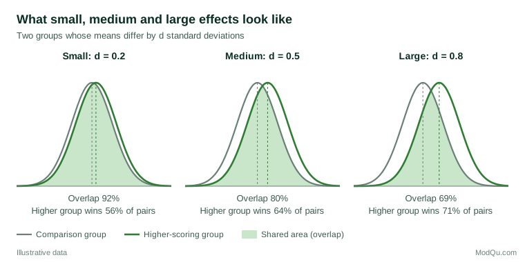
The effect size tells a more modest story. The raw difference is 0.4 points, and d = 0.4 ÷ 2.0 = 0.20. An approximate 95% confidence interval for d runs from about 0.06 to 0.34. Translated into a more intuitive form, the common-language effect size (McGraw & Wong, 1992) is 0.56: if one respondent is drawn at random from each group, the Concept A viewer gives the higher score 56% of the time, against 50% if there were no difference. The two distributions overlap by about 92%.
Whether 0.4 points matters is a business judgement, not a statistical one. If past campaigns show that each point of intent is worth a measurable share gain, a 0.4-point edge may justify choosing Concept A. If production costs differ sharply, it may not. The p-value alone could never have supported that conversation.
Interpreting magnitude
Cohen (1988, 1992) proposed rough benchmarks: d of 0.2, 0.5 and 0.8 as small, medium and large, and r of 0.10, 0.30 and 0.50. He presented them as a fallback for when nothing better is known, not as universal rules. Funder and Ozer (2019) argue that these labels are often misleading. A correlation of 0.10 can be important when an effect accumulates over many customers or many purchases, and they suggest that very large effects in real-world data should prompt suspicion rather than celebration.
Better reference points come from the context:
- Previous studies in the same category, such as typical lifts from past A/B tests or normal wave-to-wave movement in a tracker.
- Costs and benefits, such as the revenue value of a 1-point gain in conversion.
- The smallest difference anyone would act on, agreed before the data arrive.
Figure 1 is a reminder that even a "large" standardised effect leaves considerable overlap. A d of 0.8 still means that about 21% of the lower group scores above the average of the higher group.
Reporting effect sizes well
Good reporting combines the size of the effect with its uncertainty. Cumming (2014) recommends making estimates and confidence intervals, rather than significance decisions, the centre of interpretation. In practice:
- Report the raw difference in meaningful units first, then a standardised measure where it aids comparison.
- Give a confidence interval for the effect, not just the point estimate (Cumming, 2014).
- State which variant was used (d or g, pooled or control-group standard deviation, risk ratio or odds ratio).
- Use survey weights and design-aware standard errors for weighted or clustered samples.
- Report effects for non-significant results too, so that readers can see whether the data rule out important effects or are simply imprecise.
Standardised effect sizes also make results comparable across studies, which is what allows evidence to be combined in a meta-analysis (Borenstein et al., 2009).
Common mistakes
- Treating significance as importance. A tiny effect in a sample of 50,000 can have a very small p-value. Sullivan and Feinn (2012) stress that the p-value is not enough; the effect size is the main finding.
- Applying benchmarks mechanically. Calling d = 0.3 "small" without context can dismiss an effect worth millions, or inflate one worth nothing.
- Mixing up ratio measures. An odds ratio of 2 is not "twice as likely" when the outcome is common.
- Comparing standardised effects across different populations. Because d depends on the spread in the sample, a more homogeneous sample produces a larger d for the same raw difference.
- Reporting only significant effects. Selective reporting inflates the apparent size of effects across a body of work.
Key takeaways
Effect sizes answer the question every client asks: how much? Report the raw difference whenever its units mean something, add a standardised measure when comparing across scales or studies, and always attach a confidence interval. Interpret magnitude against costs, benefits and prior evidence rather than generic labels. A result that is significant but tiny, or large but imprecise, can only be recognised as such when the effect size is on the table.
References
American Psychological Association. (2020). Publication manual of the American Psychological Association (7th ed.). https://doi.org/10.1037/0000165-000
Borenstein, M., Hedges, L. V., Higgins, J. P. T., & Rothstein, H. R. (2009). Introduction to meta-analysis. Wiley. https://doi.org/10.1002/9780470743386
Cohen, J. (1988). Statistical power analysis for the behavioral sciences (2nd ed.). Routledge. https://doi.org/10.4324/9780203771587
Cohen, J. (1992). A power primer. Psychological Bulletin, 112(1), 155–159. https://doi.org/10.1037/0033-2909.112.1.155
Cumming, G. (2014). The new statistics: Why and how. Psychological Science, 25(1), 7–29. https://doi.org/10.1177/0956797613504966
Fritz, C. O., Morris, P. E., & Richler, J. J. (2012). Effect size estimates: Current use, calculations, and interpretation. Journal of Experimental Psychology: General, 141(1), 2–18. https://doi.org/10.1037/a0024338
Funder, D. C., & Ozer, D. J. (2019). Evaluating effect size in psychological research: Sense and nonsense. Advances in Methods and Practices in Psychological Science, 2(2), 156–168. https://doi.org/10.1177/2515245919847202
Hedges, L. V. (1981). Distribution theory for Glass's estimator of effect size and related estimators. Journal of Educational Statistics, 6(2), 107–128. https://doi.org/10.3102/10769986006002107
Kelley, K., & Preacher, K. J. (2012). On effect size. Psychological Methods, 17(2), 137–152. https://doi.org/10.1037/a0028086
Lakens, D. (2013). Calculating and reporting effect sizes to facilitate cumulative science: A practical primer for t-tests and ANOVAs. Frontiers in Psychology, 4, Article 863. https://doi.org/10.3389/fpsyg.2013.00863
McGraw, K. O., & Wong, S. P. (1992). A common language effect size statistic. Psychological Bulletin, 111(2), 361–365. https://doi.org/10.1037/0033-2909.111.2.361
Sullivan, G. M., & Feinn, R. (2012). Using effect size—or why the P value is not enough. Journal of Graduate Medical Education, 4(3), 279–282. https://doi.org/10.4300/JGME-D-12-00156.1
Wilkinson, L., & the Task Force on Statistical Inference. (1999). Statistical methods in psychology journals: Guidelines and explanations. American Psychologist, 54(8), 594–604. https://doi.org/10.1037/0003-066X.54.8.594