
Statistics · Descriptive statistics
Outliers: Detection, Causes and Treatment
What outliers are, why they arise, how to detect them with robust rules rather than fragile ones, and how to decide whether to correct, keep, down-weight or set aside an unusual value.
Almost every real dataset contains a few values that look out of place: a respondent who reports spending $12,000 a month on groceries, a store whose sales are ten times the regional average, a survey completed in 40 seconds. These outliers can be the most important observations in a study or the most misleading. A single extreme value can move a mean, inflate a standard deviation, reverse a regression slope and change a business decision. Deleting it without thought can be just as damaging, because some outliers carry exactly the information an analyst most needs.
This article explains what outliers are, where they come from, how to detect them reliably and how to choose a defensible treatment, with an emphasis on survey and business data.
What counts as an outlier?
There is no single formal definition. Grubbs (1969) described an outlying observation as one that appears to deviate markedly from the other members of the sample in which it occurs. Hawkins (1980) added an idea about cause: an outlier deviates so much from the other observations that it raises the suspicion it was produced by a different mechanism. The two definitions point to the two questions an analyst must answer. Is the value unusual, given the rest of the data? And if so, why?
The word "outlier" is used for several different things, and it helps to keep them apart:
- Univariate outliers are extreme on one variable, such as an unusually high income.
- Multivariate outliers are unusual in their combination of values, even if each value is ordinary on its own. A 22-year-old respondent who reports 30 years in their current job is an example.
- Contextual outliers are unusual only in a particular setting, such as high heating sales in July. Chandola et al. (2009) review this and other types in their survey of anomaly detection.
- Influential observations are points that change the results of a model when they are removed. They are not always extreme on any single variable, and an extreme point is not always influential (Cook, 1977).
Aguinis et al. (2013) reviewed the methodological literature and found 14 distinct definitions of outliers, 39 techniques for identifying them and 20 ways of handling them. They group outliers into three broad kinds that are useful in practice: error outliers, which are simply wrong; interesting outliers, which are accurate and may reveal something important; and influential outliers, which drive the results of an analysis.
Why outliers matter
Many familiar statistics are highly sensitive to a single value. The mean uses every observation with equal weight, so one large value pulls it towards itself without limit. The standard deviation is even more sensitive, because deviations are squared. Least-squares regression shares the same weakness.
The influence function, introduced by Hampel (1974), measures how much an estimate changes when a small amount of contamination is added at a given value. The breakdown point is the smallest fraction of the data that can be replaced by arbitrary values and drive the estimate to any value at all. The mean has a breakdown point of zero, because one bad value is enough, while the median can tolerate almost half of the data being contaminated (Rousseeuw & Leroy, 1987). The difference explains why the median is the standard summary for skewed variables such as income, spending and house prices.
Causes of outliers
Understanding the cause is the most important step, because the cause determines the treatment. Common causes fall into four groups.
Errors in recording and processing
Typing 1250 instead of 125.0, reporting annual income in a monthly field, mixing currencies or units, and treating a missing-value code such as 999 as a real number all create outliers that are simply wrong.
Measurement and response problems
In surveys, some respondents answer carelessly, speed through the questionnaire or give random or patterned answers. Meade and Craig (2012) showed that careless responding is common enough to distort results, and that it can be detected with a combination of indicators: response time, consistency across similar items, instructed-response items ("select 'strongly agree' for this question") and multivariate distance measures.
A different population
Sometimes an outlier is accurate but belongs to a group the study did not intend to cover, such as a business account in a consumer panel or a wholesale order in retail transaction data.
Genuine extreme values
Customer spending, company revenue and insurance claims are all highly skewed, and the largest values are real and often very important. In business surveys, a handful of very large firms can account for a large share of a total. Chambers (1986) distinguished representative outliers, which are correctly recorded and may have similar counterparts in the unsampled part of the population, from non-representative ones, which are errors or unique cases. Representative outliers should not be deleted, but they may need special handling so that they do not dominate an estimate.
Detecting outliers
No detection method tells you what to do with a flagged value; it only tells you where to look.
Look at the data first
Histograms, box plots, dot plots and scatter plots reveal most problems faster than any test. The box plot, popularised by John Tukey, marks values beyond "fences" set at 1.5 times the interquartile range (IQR) below the first quartile and above the third:
Lower fence = Q1 − 1.5 × IQR Upper fence = Q3 + 1.5 × IQR
For a normal distribution these fences sit about 2.7 standard deviations from the mean, so roughly 0.7% of values would fall outside them even with no problems in the data. Hoaglin et al. (1986) studied how this rule performs and showed that, in clean samples, it still flags at least one value fairly often, so a point beyond the fences is a prompt for inspection rather than proof of a problem. For skewed data the ordinary box plot flags too many values in the long tail. Hubert and Vandervieren (2008) proposed an adjusted box plot that shifts the fences according to a robust measure of skewness.
z-scores and their weakness
A common rule is to flag any value more than three standard deviations from the mean, that is, with |z| > 3, where:
z = (x − x̄) ÷ s
The rule is easy to apply but has a serious flaw: the mean and standard deviation are themselves distorted by the outliers it is trying to find. Large values inflate s, which shrinks every z-score and can hide other outliers. This is called masking. In small samples the rule can fail completely: with n observations, no z-score can exceed (n − 1) ÷ √n, so in a sample of 10 no value can ever pass 3.
Robust z-scores based on the median
A better approach replaces the mean with the median and the standard deviation with the median absolute deviation (MAD), the median of the absolute distances from the median. Multiplied by 1.4826, the MAD estimates the standard deviation for normal data while staying resistant to outliers:
Robust z = (x − median) ÷ (1.4826 × MAD)
Leys et al. (2013) argued that the standard-deviation rule should be abandoned in favour of this one and suggested a threshold of 2.5 as a reasonable default. Rousseeuw and Croux (1993) proposed alternative robust scale estimators that keep the MAD's resistance while being more efficient.
Formal tests
Classical outlier tests assume the data are otherwise normal. Grubbs' test asks whether the most extreme value is too far from the mean to be plausible (Grubbs, 1950, 1969). Dixon's test uses the gaps between ordered values and was designed for small samples (Dixon, 1950). Both test for one outlier at a time, and repeating them can suffer from masking. The generalised extreme studentised deviate procedure of Rosner (1983) tests for up to a pre-specified number of outliers while controlling the overall error rate. They suit roughly normal laboratory and quality-control data better than skewed business variables.
Multivariate and model-based detection
For several variables at once, the Mahalanobis distance measures how far each observation lies from the centre of the data, allowing for correlations between variables. Like the z-score, it is distorted when the mean and covariance matrix are estimated from contaminated data. Robust versions based on the minimum covariance determinant (MCD) estimator, made practical by the fast algorithm of Rousseeuw and Van Driessen (1999), solve this problem. Rousseeuw and van Zomeren (1990) showed how robust distances can unmask multivariate outliers and leverage points that classical methods miss.
In regression, three diagnostics work together. Residuals show points the model fits poorly. Leverage shows points with unusual predictor values. Cook's distance combines the two to measure how much the fitted model changes when each observation is removed (Cook, 1977). Rousseeuw and Leroy (1987) describe robust regression methods that fit the bulk of the data and expose the points that do not follow it.
For very large datasets, such as transaction logs, algorithmic methods such as the isolation forest are common: it flags points that random splits of the data isolate unusually quickly (Liu et al., 2008). A human still has to judge what the flagged cases mean.
A worked example
Suppose a hypothetical survey asks 20 households for their weekly grocery spending. The answers, in dollars, are:
62, 74, 81, 88, 93, 97, 102, 105, 110, 114, 118, 121, 127, 133, 139, 146, 158, 172, 420 and 1,250.
The mean is $185.50 and the standard deviation is $261.22, while the median is $116. Applying the three-standard-deviation rule, the value 1,250 has z = 4.08 and is flagged, but 420 has z = 0.90 and looks unremarkable. The large value has inflated the standard deviation enough to mask the second one.
The robust rules tell a different story. The quartiles are 96.0 and 140.75, so the IQR is 44.75 and the upper Tukey fence is 207.9. The MAD is 23, giving a robust standard deviation of 34.1 and an upper limit of 201.2 at 2.5 robust z-units. Both rules flag 420 and 1,250, and nothing else.
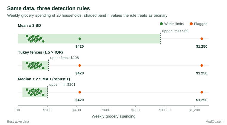
Investigation then matters more than detection. Checking the source shows that 1,250 was a keying error for 125.0. Once it is corrected, the mean falls to $129.25 and the standard deviation to $73.87, and the 420 now has z = 3.94: the masking has disappeared. The 420 turns out to be a real answer from a household of seven that shops for an extended family. It is accurate, so it stays in the data. The median, $116, did not change at any point.
Treating outliers
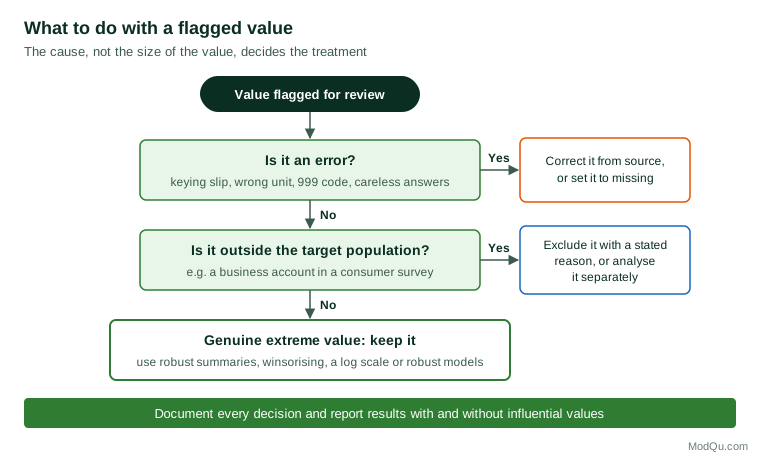
The right treatment follows from the cause. Figure 2 summarises the main decisions.
Correct or remove errors
Values that are demonstrably wrong should be corrected from the source if possible, for example by checking the original form or recontacting the respondent. If the true value cannot be recovered, set it to missing and handle it like other missing data. Careless or fraudulent survey responses are normally removed as whole cases, using rules set before fieldwork.
Keep genuine values, but limit their influence
Deleting accurate data because it is inconvenient biases results and understates variability. When an extreme value is real, there are better options:
- Report robust summaries. The median, the trimmed mean (which drops a fixed percentage of values from each end) and M-estimators, which down-weight extreme values smoothly, were developed for exactly this purpose (Huber, 1964, 1981). In the uncorrected example, the 10% trimmed mean is $119.00, close to the median and far from the raw mean.
- Winsorise. Winsorising replaces values beyond a chosen percentile with the value at that percentile, rather than deleting them. Winsorising the two lowest and two highest values in the uncorrected example gives a mean of $120.50. In business surveys, winsorising very large reported values is a common way to stop a few units dominating an estimated total, at the cost of a small bias (Chambers, 1986).
- Transform the variable. A log transformation often makes a skewed variable roughly symmetric.
- Use robust models. Robust regression and quantile regression reduce the pull of extreme points on a fitted line (Rousseeuw & Leroy, 1987).
Exclude values from outside the population, openly
Cases that belong to a different population can be excluded from the main analysis, but the reason should be stated and the rule applied consistently. Sometimes they deserve their own analysis: a small group of very heavy buyers may be the most valuable segment in the market.
Decide in advance and report both ways
Anscombe (1960) compared outlier rejection rules to an insurance policy: they protect against the damage caused by bad values, but there is a premium, paid in lost efficiency when the extreme values were genuine. The way to keep that trade-off honest is to set the rules in advance. Leys et al. (2019) recommend that researchers decide and pre-register how outliers will be detected and managed before seeing the results. Aguinis et al. (2013) recommend reporting results with and without influential observations so that readers can judge how much depends on them.
Practical guidance for survey and business data
- Build checks into the questionnaire. Range checks, unit prompts ("per week or per month?") and confirmation messages for unusual entries prevent many error outliers at the source.
- Screen for careless responding before analysis. Combine completion time, straight-lining, failed attention checks and inconsistent answers rather than relying on one indicator (Meade & Craig, 2012).
- Use robust rules for screening. Prefer quartile or median-based rules, or the adjusted box plot for skewed variables, to the three-standard-deviation rule.
- Look at weighted values. In a weighted survey, an ordinary answer from a respondent with a very large weight can be influential. Check the product of value and weight, not just the value.
- Check segments separately. An outlier in a small subgroup can distort that group's estimates even when it is invisible in the total.
- Keep an audit trail. Record every flagged value, the reason for the decision and its effect on the key results.
Common mistakes
- Automatic deletion. Removing every value beyond a cut-off without investigation discards real information and can make variation look smaller than it is.
- Relying on the mean and standard deviation to find outliers. As the example shows, these statistics are distorted by the very values they are meant to detect.
- Repeating deletion until the data look clean. Each round finds new "outliers" and gradually trims the tails of a genuinely skewed distribution.
- Choosing the rule after seeing the results. Trying several treatments and reporting the one that gives the preferred answer is a form of selective reporting.
- Ignoring multivariate outliers. Inconsistent combinations of answers often reveal careless responses that univariate checks miss.
- Confusing extreme with influential. A point can be extreme without changing the result, and a moderate point can change a regression substantially. Diagnostics such as Cook's distance address influence directly.
Key takeaways
Outliers are a signal to investigate, not a problem to delete. Detect them with plots and robust rules based on quartiles or the median, not with the mean and standard deviation. Then find the cause: correct or remove errors, set aside cases from outside the target population with a stated reason, and keep genuine extreme values while limiting their influence through robust summaries, winsorising, transformation or robust models. Decide the rules before the analysis, document every decision, and show how much the results depend on the unusual values.
References
Aguinis, H., Gottfredson, R. K., & Joo, H. (2013). Best-practice recommendations for defining, identifying, and handling outliers. Organizational Research Methods, 16(2), 270–301. https://doi.org/10.1177/1094428112470848
Anscombe, F. J. (1960). Rejection of outliers. Technometrics, 2(2), 123–146. https://doi.org/10.1080/00401706.1960.10489888
Chambers, R. L. (1986). Outlier robust finite population estimation. Journal of the American Statistical Association, 81(396), 1063–1069. https://doi.org/10.1080/01621459.1986.10478374
Chandola, V., Banerjee, A., & Kumar, V. (2009). Anomaly detection. ACM Computing Surveys, 41(3), 1–58. https://doi.org/10.1145/1541880.1541882
Cook, R. D. (1977). Detection of influential observation in linear regression. Technometrics, 19(1), 15–18. https://doi.org/10.1080/00401706.1977.10489493
Dixon, W. J. (1950). Analysis of extreme values. The Annals of Mathematical Statistics, 21(4), 488–506. https://doi.org/10.1214/aoms/1177729747
Grubbs, F. E. (1950). Sample criteria for testing outlying observations. The Annals of Mathematical Statistics, 21(1), 27–58. https://doi.org/10.1214/aoms/1177729885
Grubbs, F. E. (1969). Procedures for detecting outlying observations in samples. Technometrics, 11(1), 1–21. https://doi.org/10.1080/00401706.1969.10490657
Hampel, F. R. (1974). The influence curve and its role in robust estimation. Journal of the American Statistical Association, 69(346), 383–393. https://doi.org/10.1080/01621459.1974.10482962
Hawkins, D. M. (1980). Identification of outliers. Springer. https://doi.org/10.1007/978-94-015-3994-4
Hoaglin, D. C., Iglewicz, B., & Tukey, J. W. (1986). Performance of some resistant rules for outlier labeling. Journal of the American Statistical Association, 81(396), 991–999. https://doi.org/10.1080/01621459.1986.10478363
Huber, P. J. (1964). Robust estimation of a location parameter. The Annals of Mathematical Statistics, 35(1), 73–101. https://doi.org/10.1214/aoms/1177703732
Huber, P. J. (1981). Robust statistics. Wiley. https://doi.org/10.1002/0471725250
Hubert, M., & Vandervieren, E. (2008). An adjusted boxplot for skewed distributions. Computational Statistics & Data Analysis, 52(12), 5186–5201. https://doi.org/10.1016/j.csda.2007.11.008
Leys, C., Delacre, M., Mora, Y. L., Lakens, D., & Ley, C. (2019). How to classify, detect, and manage univariate and multivariate outliers, with emphasis on pre-registration. International Review of Social Psychology, 32(1), Article 5. https://doi.org/10.5334/irsp.289
Leys, C., Ley, C., Klein, O., Bernard, P., & Licata, L. (2013). Detecting outliers: Do not use standard deviation around the mean, use absolute deviation around the median. Journal of Experimental Social Psychology, 49(4), 764–766. https://doi.org/10.1016/j.jesp.2013.03.013
Liu, F. T., Ting, K. M., & Zhou, Z.-H. (2008). Isolation forest. In 2008 Eighth IEEE International Conference on Data Mining (pp. 413–422). IEEE. https://doi.org/10.1109/ICDM.2008.17
Meade, A. W., & Craig, S. B. (2012). Identifying careless responses in survey data. Psychological Methods, 17(3), 437–455. https://doi.org/10.1037/a0028085
Rosner, B. (1983). Percentage points for a generalized ESD many-outlier procedure. Technometrics, 25(2), 165–172. https://doi.org/10.1080/00401706.1983.10487848
Rousseeuw, P. J., & Croux, C. (1993). Alternatives to the median absolute deviation. Journal of the American Statistical Association, 88(424), 1273–1283. https://doi.org/10.1080/01621459.1993.10476408
Rousseeuw, P. J., & Leroy, A. M. (1987). Robust regression and outlier detection. Wiley. https://doi.org/10.1002/0471725382
Rousseeuw, P. J., & Van Driessen, K. (1999). A fast algorithm for the minimum covariance determinant estimator. Technometrics, 41(3), 212–223. https://doi.org/10.1080/00401706.1999.10485670
Rousseeuw, P. J., & van Zomeren, B. C. (1990). Unmasking multivariate outliers and leverage points. Journal of the American Statistical Association, 85(411), 633–639. https://doi.org/10.1080/01621459.1990.10474920