
Statistics · Tests and models
Ordinal and Multinomial Regression for Survey Responses
How ordinal and multinomial regression model survey answers with more than two categories, how to read their results as predicted probabilities, and which assumptions to check before reporting them.
Many survey questions have more than two possible answers. Some are ordered, such as a five-point scale from "very unlikely" to "very likely" to renew. Others are unordered, such as a respondent's preferred brand or main reason for cancelling. Linear regression treats the first kind as if the gaps between categories were equal, and logistic regression handles only two outcomes. Ordinal and multinomial regression extend logistic regression to these cases (Agresti, 2010; Hosmer et al., 2013).
Ordinal regression
The most common ordinal model is the proportional odds (cumulative logit) model popularised by McCullagh (1980). For an outcome with categories 1 to J, it models the log-odds of answering at or below each category j:
log[P(Y ≤ j) ÷ P(Y > j)] = θj − βx, for j = 1, …, J − 1
Each cut-point θj marks a threshold between adjacent categories, while a single coefficient β describes how the predictor shifts the whole distribution up or down the scale. A useful way to picture the model is a continuous latent attitude, such as willingness to renew, that respondents translate into the nearest available answer.
A worked example
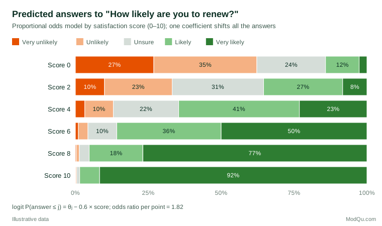
Suppose a hypothetical survey asks customers how likely they are to renew, on a five-point scale, and also records their satisfaction from 0 to 10. A proportional odds model gives β = 0.6. Exponentiating gives an odds ratio of e0.6 ≈ 1.82: each extra satisfaction point multiplies the odds of giving a more positive answer, at any cut-point, by about 1.8. This one number applies equally to the odds of "likely or very likely" versus the rest and to the odds of anything above "very unlikely".
Odds ratios are not intuitive for most audiences, so it is better to report predicted probabilities (Figure 1). At a satisfaction score of 0, the model predicts that 14% of customers will say they are likely or very likely to renew; at 5 the figure is 77%, and at 10 it is 99%. The cut-points (here −1.0, 0.5, 1.8 and 3.6 on the log-odds scale) rarely need to be reported in their own right; they simply fix where the category boundaries fall. Note also that the shifts are not equal on the probability scale: the same coefficient moves predictions most in the middle of the scale.
Why not just use linear regression?
Treating a rating scale as numeric and running ordinary regression is common and often gives similar conclusions. But it assumes equal spacing between categories, can predict impossible values, and ignores ceiling and floor effects. Liddell and Kruschke (2018) showed with real and simulated data that analysing ordinal ratings as if they were metric can produce false alarms, missed differences and even reversed effects, particularly when groups differ in variability. Jamieson (2004) made the more general point that the intervals between response categories cannot be presumed equal. Ordinal models avoid these problems, and modern tutorials such as Bürkner and Vuorre (2019) show how to fit and interpret them, including related forms such as sequential and adjacent-category models.
The proportional odds assumption
The model's simplicity comes from assuming that a predictor has the same effect at every cut-point. If, for example, satisfaction strongly separates "very unlikely" from the rest but barely separates "likely" from "very likely", the assumption fails. The Brant (1990) test checks it formally, although with large samples it flags trivial departures, so plots of separate binary logits at each cut-point are a useful complement. When the assumption fails for some predictors, a partial proportional odds or generalised ordered logit model lets those effects vary across cut-points while keeping the rest constant (Williams, 2006).
Multinomial regression
When categories have no natural order, multinomial (polytomous) logistic regression compares each category with a chosen reference category:
log[P(Y = k) ÷ P(Y = reference)] = β0k + β1kx, for each k ≠ reference
A question with four brands therefore produces three sets of coefficients. Exponentiated coefficients are often called relative risk ratios, and again predicted probabilities are usually the clearest summary: for instance, how the predicted share preferring each brand changes with age or income.
Multinomial models rest on the assumption of independence of irrelevant alternatives: the relative odds of choosing between two options should not depend on whether other options are available. If adding a close substitute to the list draws respondents mainly from one competitor, the assumption is violated. Hausman and McFadden (1984) proposed a widely used test, and nested or mixed logit models relax the assumption.
Practical guidance
- Choose the model from the question. Use ordinal models for ordered scales, multinomial models for unordered choices. Fitting a multinomial model to an ordered scale is valid but wastes information and multiplies the number of coefficients.
- Watch sparse categories. Categories chosen by few respondents give unstable estimates. Combining adjacent categories can help, but decide this before seeing results.
- Report probabilities. Present predicted probabilities or average marginal effects for typical profiles, not only odds ratios.
- Use survey weights and design-aware standard errors for complex samples, as with any regression.
- Remember the limits. Like other regression models fitted to survey data, these models show associations, not causes.
Key takeaways
Ordinal and multinomial regression are the natural models for survey answers with more than two categories. The proportional odds model summarises a predictor's effect on an ordered scale with one coefficient, provided its central assumption holds; multinomial models handle unordered choices at the cost of more coefficients and the independence assumption. In both cases, predicted probabilities make the results clear to decision-makers.
References
Agresti, A. (2010). Analysis of ordinal categorical data (2nd ed.). Wiley. https://doi.org/10.1002/9780470594001
Brant, R. (1990). Assessing proportionality in the proportional odds model for ordinal logistic regression. Biometrics, 46(4), 1171–1178. https://doi.org/10.2307/2532457
Bürkner, P.-C., & Vuorre, M. (2019). Ordinal regression models in psychology: A tutorial. Advances in Methods and Practices in Psychological Science, 2(1), 77–101. https://doi.org/10.1177/2515245918823199
Hausman, J. A., & McFadden, D. (1984). Specification tests for the multinomial logit model. Econometrica, 52(5), 1219–1240. https://doi.org/10.2307/1910997
Hosmer, D. W., Jr., Lemeshow, S., & Sturdivant, R. X. (2013). Applied logistic regression (3rd ed.). Wiley. https://doi.org/10.1002/9781118548387
Jamieson, S. (2004). Likert scales: How to (ab)use them. Medical Education, 38(12), 1217–1218. https://doi.org/10.1111/j.1365-2929.2004.02012.x
Liddell, T. M., & Kruschke, J. K. (2018). Analyzing ordinal data with metric models: What could possibly go wrong? Journal of Experimental Social Psychology, 79, 328–348. https://doi.org/10.1016/j.jesp.2018.08.009
McCullagh, P. (1980). Regression models for ordinal data. Journal of the Royal Statistical Society Series B: Statistical Methodology, 42(2), 109–127. https://doi.org/10.1111/j.2517-6161.1980.tb01109.x
Williams, R. (2006). Generalized ordered logit/partial proportional odds models for ordinal dependent variables. The Stata Journal, 6(1), 58–82. https://doi.org/10.1177/1536867X0600600104