
Statistics · Tests and models
Correlation Is Not Causation: Spurious Relationships in Data
The main ways a correlation can appear without a causal link, with classic examples, a visual guide to Simpson's paradox, and practical checks before acting on a relationship in data.
"Correlation is not causation" may be the best-known phrase in statistics. Almost everyone agrees with it, and yet business reports, news stories and even scientific papers regularly treat associations as if they were proof of cause and effect. The phrase is also incomplete: correlation is often evidence of causation, and some of the most important discoveries in medicine began as correlations. The useful question is not whether a correlation proves causation, but what else could explain it, and how those explanations can be ruled out. This article sets out the main ways spurious relationships arise and the checks that guard against them.
What a correlation tells us
A correlation coefficient measures how closely two variables move together, on a scale from −1 to +1. A value near zero means there is no linear relationship; a value near ±1 means the points fall almost on a straight line. A correlation summarises a pattern in the data. It says nothing on its own about why the pattern exists.
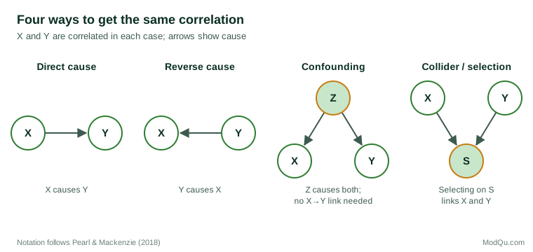
When two variables X and Y are correlated, there are at least five possible explanations:
- X causes Y.
- Y causes X (reverse causation).
- A third factor causes both (confounding).
- The way the data were selected created the relationship (selection or collider bias).
- The relationship is a coincidence or an artefact of trends over time (chance and spurious trends).
Only the first is the causal story we usually want to tell. The rest are the subject of this article.
Confounding: the hidden third factor
Confounding occurs when a third variable influences both of the variables being studied. Ice cream sales and drowning deaths both rise in summer, not because one causes the other, but because hot weather increases both swimming and ice cream consumption.
A more serious example comes from medicine. For many years, observational studies found that women who took hormone replacement therapy after menopause had lower rates of heart disease, and the therapy was widely prescribed partly for that reason. When the Women's Health Initiative tested the therapy in a large randomised controlled trial, the combination of oestrogen and progestin was found to increase the risk of coronary heart disease, stroke and breast cancer, and the trial was stopped early (Writing Group for the Women's Health Initiative Investigators, 2002). The apparent benefit in observational data was largely explained by the kind of women who chose to take the therapy, who tended to be healthier and better off to begin with.
Confounding can produce absurd correlations as well as dangerous ones. Messerli (2012) reported a strong correlation (r = 0.79) between countries' chocolate consumption per person and their number of Nobel laureates per 10 million people across 23 countries. The paper was written partly tongue in cheek, but it illustrates the point: national wealth and investment in research and education plausibly drive both.
Simpson's paradox
Confounding can be strong enough to reverse the direction of a relationship. This is Simpson's paradox, described formally by Simpson (1951): a trend that appears within every subgroup of the data can disappear or reverse when the groups are combined.
The best-known example concerns graduate admissions at the University of California, Berkeley, in 1973. Across the university as a whole, men were admitted at a noticeably higher rate than women, which suggested bias against women. When Bickel et al. (1975) examined admissions department by department, they found no general pattern of bias against women; if anything, several departments slightly favoured women. The overall difference arose because women more often applied to departments that were highly competitive and admitted a low share of all applicants, while men more often applied to departments with high admission rates.
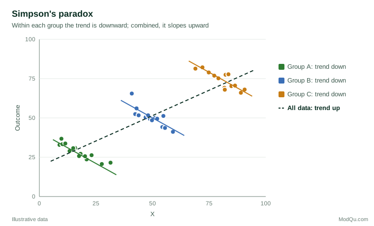
Simpson's paradox shows that no amount of data can decide, on its own, whether the combined or the separated figures give the right answer. That depends on the causal structure (Pearl, 2009): on whether the grouping variable is a confounder that should be controlled for, or a consequence of the factor being studied, which should not (Pearl & Mackenzie, 2018).
Reverse causation
Sometimes the cause runs the opposite way from what is assumed. Companies that spend more on customer service may have more complaints, not because service causes complaints, but because a large volume of complaints leads them to hire more staff. People who use a fitness app may be fitter, partly because fitter people are more likely to download one. Time order is the first check: a cause must come before its effect. Hill (1965) listed temporality as the one consideration that is essential before an association can be judged causal.
Selection and collider bias
A correlation can also be created by the way data are collected. If two independent factors both make it more likely that a case enters the dataset, then within that dataset they will appear related. Berkson (1946) described this in hospital data: because patients are admitted when they have one condition or another, two diseases that are unrelated in the general population can appear associated among hospital patients.
The same mechanism affects business data. Suppose a company surveys only customers who contacted its help desk. Customers contact the help desk either because the product is complex or because they are inexperienced. Among those who called, product complexity and user experience may then appear negatively related even if they are unrelated in the customer base. In causal diagrams, the selection variable is called a collider, because two arrows collide in it, and controlling for a collider creates bias rather than removing it (Elwert & Winship, 2014; Hernán et al., 2004).
For survey research, the lesson is that who answers can shape the relationships found, not just the averages. Opt-in samples, customer panels and website visitors are all selected groups.
Chance and spurious trends
With enough variables, some will be correlated by chance. A business that tests hundreds of possible drivers of sales will find several that appear significant at the 5% level even if none has any real effect. Procedures that control the false discovery rate limit how many such findings are mistaken for real effects (Benjamini & Hochberg, 1995).
Ratios create a related trap. Pearson (1897) showed that two unrelated measurements become correlated when both are divided by the same third quantity, as with sales per employee and costs per employee.
Data recorded over time pose a special problem. Any two series that both trend upwards or downwards will be correlated, whatever their connection. Yule (1926) gave a famous example: between 1866 and 1911, the proportion of marriages in England and Wales conducted by the Church of England was very highly correlated (about 0.95) with the mortality rate. Neither caused the other; both were declining over the same period. Granger and Newbold (1974) later showed that regressions between unrelated trending series routinely produce apparently strong and significant results, and that such results should be treated with suspicion unless the trends are accounted for.
How spurious relationships appear in business data
The same mechanisms appear constantly in commercial analysis. Three common situations illustrate them.
The loyalty programme. A retailer finds that members of its loyalty programme spend far more each year than non-members and concludes that the programme drives spending. But customers who already shop often are the ones most likely to join, so the comparison mixes the effect of the programme with the effect of prior loyalty. This is a combination of confounding and reverse causation. A fairer test compares the same customers' spending before and after joining, against similar customers who did not join over the same period, or offers membership to a randomly chosen group.
The satisfaction driver. A survey shows that customers who rate the help desk highly are also more likely to renew their contracts. It is tempting to conclude that improving the help desk will increase renewals. Yet customers who are happy with the product overall tend to rate every part of the service more generously, a general positive impression that affects all their answers. Some of the correlation reflects that overall impression rather than any specific effect of the help desk. Driver analyses based on survey ratings should therefore be treated as hypotheses about where to act, to be tested where possible.
The marketing campaign. Website traffic and sales both rise sharply in the weeks after a campaign launches, and the campaign is credited with the increase. If the campaign was timed to coincide with a seasonal peak, the season may explain much of the rise. Comparing results with the same period in previous years, or with regions where the campaign did not run, helps separate the effect of the campaign from the effect of the calendar.
In each case the correlation is real and the causal story is plausible, but it is not the only story the data can tell. The task of analysis is to test the alternatives before acting.
How strong is strong?
A related mistake is to treat the size of a correlation as a measure of how much one variable affects another. A correlation of 0.3 is common in social and business data and may reflect a real and useful relationship, yet it means that only about 9% of the variation in one variable is shared with the other (the square of the correlation). Conversely, a very high correlation, like Yule's 0.95, may have no causal meaning at all. The strength of a correlation describes how tightly the points cluster around a line, not how large an effect a change in one variable would have on the other, and not whether there is any effect.
Correlations can also hide relationships. A correlation coefficient measures only linear association. If an outcome rises and then falls as a variable increases, as customer satisfaction might with the number of contacts from a sales team, the correlation can be close to zero even though the relationship is strong. Plotting the data before calculating any statistic is the simplest protection against both errors; Anscombe (1973) showed that four datasets with the same correlation can look entirely different when plotted.
Correlations between groups can also mislead about individuals. Robinson (1950) showed that correlations calculated across US regions could be far stronger than, and even opposite in sign to, the corresponding correlations between individuals.
From correlation to causation
If correlation alone cannot prove causation, how are causal conclusions reached? Several approaches help.
Randomised experiments. Random assignment breaks the link between the treatment and every possible confounder, measured or not. A causal effect is the difference between what happens to the same unit with and without the treatment, which can never be observed directly; randomisation allows it to be estimated on average (Holland, 1986; Rubin, 1974). This is why randomised controlled trials and online A/B tests (Kohavi et al., 2009) are considered the strongest evidence of cause and effect, and why the Women's Health Initiative trial could overturn decades of observational findings.
Causal reasoning about the data. Where experiments are impossible, researchers can draw an explicit causal diagram of how they believe the variables relate, decide which variables must be controlled for and which must not, and test the implications (Pearl & Mackenzie, 2018).
Natural experiments. Designs such as difference-in-differences and instrumental variables use situations in which a treatment was assigned almost as if at random (Angrist & Pischke, 2009).
Weighing the evidence. Hill (1965) proposed a set of considerations for judging whether an observed association is likely to be causal: its strength, its consistency across studies, its specificity, temporality, a dose–response gradient, plausibility, coherence with other knowledge, experimental evidence and analogy. Hill stressed that these are aids to judgement, not a checklist that proves causation. They were developed in the context of the evidence linking smoking with lung cancer (Doll & Hill, 1950). Cornfield et al. (1959) showed that any confounder would need an implausibly strong link with smoking to explain that association away. It is a case in which observational correlations, carefully examined, rightly led to a causal conclusion.
Practical checks before acting on a correlation
Before treating a relationship in data as a reason to act, it is worth asking:
- Which came first? Check the time order of cause and effect.
- What else could drive both? List plausible confounders and see whether the relationship survives when they are accounted for.
- How were the data selected? Ask whether the sample was filtered in a way that could create the relationship.
- Does it hold within subgroups? Look for Simpson's paradox by breaking the data down by key segments.
- Are both series trending? For data over time, examine changes rather than levels, or remove the trends.
- How many relationships were tested? Adjust expectations for the number of comparisons made.
- Can it be tested? Where possible, run an experiment, even a small one, before making a large investment.
Reporting relationships responsibly
Even when a causal conclusion cannot be reached, a correlation can still be worth reporting. The key is to describe it accurately. Phrases such as "is associated with", "is more common among" and "tends to occur alongside" describe what the data show. Phrases such as "leads to", "drives", "boosts" and "causes" make a causal claim that needs causal evidence. Reports that use survey or transactional data should say which kind of claim they are making, mention the most plausible alternative explanations, and indicate what further evidence, such as an experiment, would settle the question. Readers can then judge for themselves how much weight to place on the finding, and decision-makers can match the size of their bet to the strength of the evidence.
Conclusion
Correlations are the raw material of discovery, but they are not conclusions. A relationship in data may reflect cause and effect, a hidden third factor, a reversed arrow, the way the sample was drawn, or simple coincidence. The tools for telling these apart, including experiments, causal diagrams and careful judgement, are what turn statistical patterns into knowledge that can safely guide decisions.
References
Angrist, J. D., & Pischke, J.-S. (2009). Mostly harmless econometrics: An empiricist's companion. Princeton University Press. https://doi.org/10.1515/9781400829828
Anscombe, F. J. (1973). Graphs in statistical analysis. The American Statistician, 27(1), 17–21. https://doi.org/10.1080/00031305.1973.10478966
Benjamini, Y., & Hochberg, Y. (1995). Controlling the false discovery rate: A practical and powerful approach to multiple testing. Journal of the Royal Statistical Society: Series B (Methodological), 57(1), 289–300. https://doi.org/10.1111/j.2517-6161.1995.tb02031.x
Berkson, J. (1946). Limitations of the application of fourfold table analysis to hospital data. Biometrics Bulletin, 2(3), 47–53. https://doi.org/10.2307/3002000
Bickel, P. J., Hammel, E. A., & O'Connell, J. W. (1975). Sex bias in graduate admissions: Data from Berkeley. Science, 187(4175), 398–404. https://doi.org/10.1126/science.187.4175.398
Cornfield, J., Haenszel, W., Hammond, E. C., Lilienfeld, A. M., Shimkin, M. B., & Wynder, E. L. (1959). Smoking and lung cancer: Recent evidence and a discussion of some questions. Journal of the National Cancer Institute, 22(1), 173–203. https://doi.org/10.1093/jnci/22.1.173
Doll, R., & Hill, A. B. (1950). Smoking and carcinoma of the lung. British Medical Journal, 2(4682), 739–748. https://doi.org/10.1136/bmj.2.4682.739
Elwert, F., & Winship, C. (2014). Endogenous selection bias: The problem of conditioning on a collider variable. Annual Review of Sociology, 40, 31–53. https://doi.org/10.1146/annurev-soc-071913-043455
Granger, C. W. J., & Newbold, P. (1974). Spurious regressions in econometrics. Journal of Econometrics, 2(2), 111–120. https://doi.org/10.1016/0304-4076(74)90034-7
Hernán, M. A., Hernández-Díaz, S., & Robins, J. M. (2004). A structural approach to selection bias. Epidemiology, 15(5), 615–625. https://doi.org/10.1097/01.ede.0000135174.63482.43
Hill, A. B. (1965). The environment and disease: Association or causation? Proceedings of the Royal Society of Medicine, 58(5), 295–300. https://doi.org/10.1177/003591576505800503
Holland, P. W. (1986). Statistics and causal inference. Journal of the American Statistical Association, 81(396), 945–960. https://doi.org/10.1080/01621459.1986.10478354
Kohavi, R., Longbotham, R., Sommerfield, D., & Henne, R. M. (2009). Controlled experiments on the web: Survey and practical guide. Data Mining and Knowledge Discovery, 18(1), 140–181. https://doi.org/10.1007/s10618-008-0114-1
Messerli, F. H. (2012). Chocolate consumption, cognitive function, and Nobel laureates. New England Journal of Medicine, 367(16), 1562–1564. https://doi.org/10.1056/NEJMon1211064
Pearl, J. (2009). Causality: Models, reasoning, and inference (2nd ed.). Cambridge University Press. https://doi.org/10.1017/CBO9780511803161
Pearl, J., & Mackenzie, D. (2018). The book of why: The new science of cause and effect. Basic Books.
Pearson, K. (1897). Mathematical contributions to the theory of evolution: On a form of spurious correlation which may arise when indices are used in the measurement of organs. Proceedings of the Royal Society of London, 60, 489–498. https://doi.org/10.1098/rspl.1896.0076
Robinson, W. S. (1950). Ecological correlations and the behavior of individuals. American Sociological Review, 15(3), 351–357. https://doi.org/10.2307/2087176
Rubin, D. B. (1974). Estimating causal effects of treatments in randomized and nonrandomized studies. Journal of Educational Psychology, 66(5), 688–701. https://doi.org/10.1037/h0037350
Simpson, E. H. (1951). The interpretation of interaction in contingency tables. Journal of the Royal Statistical Society: Series B (Methodological), 13(2), 238–241. https://doi.org/10.1111/j.2517-6161.1951.tb00088.x
Writing Group for the Women's Health Initiative Investigators. (2002). Risks and benefits of estrogen plus progestin in healthy postmenopausal women: Principal results from the Women's Health Initiative randomized controlled trial. JAMA, 288(3), 321–333. https://doi.org/10.1001/jama.288.3.321
Yule, G. U. (1926). Why do we sometimes get nonsense-correlations between time-series? A study in sampling and the nature of time-series. Journal of the Royal Statistical Society, 89(1), 1–63. https://doi.org/10.2307/2341482