
Statistics · Tests and models
Nonparametric Regression and Smoothing Techniques for Flexible Knowledge Representation
How smoothers such as LOESS, splines and generalised additive models let the data show the shape of a relationship, and how to choose the amount of smoothing without chasing noise.
Ordinary regression asks the analyst to decide the shape of a relationship before looking at the data: a straight line, perhaps a quadratic. Many business relationships do not follow such a neat formula. Satisfaction may hold steady while delivery is quick, then fall sharply once waiting passes a threshold. Nonparametric regression estimates the curve directly from the data, assuming only that it is reasonably smooth (Wasserman, 2006).
The idea of a smoother
A smoother estimates the average outcome at each value of a predictor by borrowing information from nearby observations. Three families dominate applied work.
- Local regression (LOESS). At each target point, a straight line is fitted to the nearest fraction of the data, with closer points weighted more heavily. The fitted values at all points are then joined into a curve. Cleveland (1979) introduced the method together with a robust version that reduces the pull of outliers.
- Smoothing splines and penalised splines. The curve is built from flexible polynomial pieces, and a penalty discourages excessive wiggliness. Eilers and Marx (1996) showed that combining many B-spline pieces with a simple difference penalty gives a fast, stable smoother.
- Generalised additive models (GAMs). These combine several smooth terms, one per predictor, inside a regression framework that can also handle binary or count outcomes. They keep the readability of regression while letting each effect bend (Wood, 2017).
The smoothing parameter
Every smoother has a dial that controls flexibility: the span in LOESS, the penalty weight in a spline. A small span lets the curve follow every local fluctuation, giving low bias but high variance. A large span averages over wide stretches of data, giving a stable curve that may flatten real features. This is the classic bias-variance trade-off (Hastie et al., 2009).
The dial should not be set by eye alone. Cross-validation chooses the value that best predicts observations left out of the fit, and generalised cross-validation offers a fast approximation for splines (Craven & Wahba, 1978). Modern GAM software selects penalties automatically by similar criteria (Wood, 2017).
A worked example
Suppose a hypothetical retailer surveys 200 customers about their satisfaction, on a 0 to 10 scale, and links each answer to the number of days the order took to arrive. Figure 1 shows three fits to the same data.
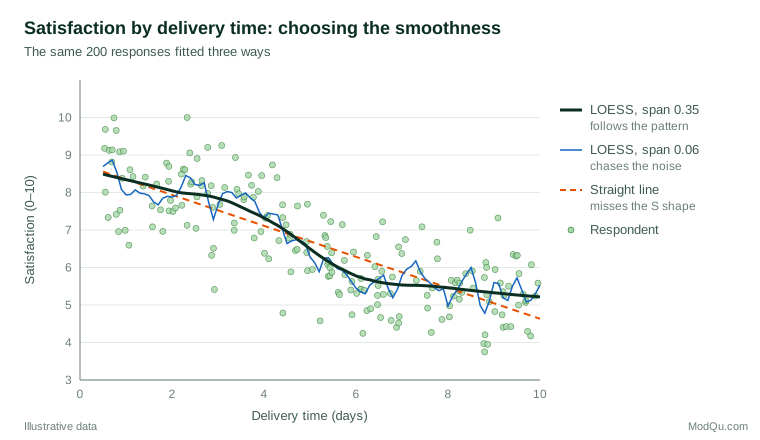
The straight line reports that each extra day costs about 0.4 points. That average hides the real story. The LOESS curve with a span of 0.35 shows satisfaction near 8.3 for next-day delivery and still about 7.8 at three days, then a drop to about 5.8 by day six, after which further delay changes little. The operational lesson is quite different: the critical window is days three to six, not every day equally. The very small span, by contrast, produces bumps that would vanish in a new sample.
Practical guidance for survey and business data
- Explore before you model. A smoother added to a scatter plot is one of the quickest checks on whether a linear term is adequate.
- Show uncertainty. Plot confidence bands, which widen where data are sparse, especially at the edges of the range.
- Use weights where needed. Most smoothing software accepts survey weights; standard errors still need design-aware methods.
- Translate the curve. Report thresholds and plateaus in plain language, as in the delivery example.
Limitations and common mistakes
- Too many predictors. Smoothing in many dimensions at once needs enormous samples, a problem known as the curse of dimensionality (Hastie et al., 2009). Additive models sidestep it by smoothing one predictor at a time, at the price of missing some interactions.
- Reading meaning into wiggles. Small bumps are often noise. Check whether they survive a sensible span and a confidence band.
- Extrapolating. A smoother says nothing reliable beyond the observed range of the predictor.
- Forgetting causation. A flexible curve is still a description of association, not proof that changing the predictor would change the outcome.
Key takeaways
Nonparametric regression lets the data reveal shapes that a fixed formula would hide, such as thresholds and plateaus. LOESS, penalised splines and GAMs are the main tools. Their usefulness depends on choosing the smoothing parameter by cross-validation rather than by eye, showing uncertainty, and interpreting only features that are large enough to matter.
References
Cleveland, W. S. (1979). Robust locally weighted regression and smoothing scatterplots. Journal of the American Statistical Association, 74(368), 829–836. https://doi.org/10.1080/01621459.1979.10481038
Craven, P., & Wahba, G. (1978). Smoothing noisy data with spline functions: Estimating the correct degree of smoothing by the method of generalized cross-validation. Numerische Mathematik, 31(4), 377–403. https://doi.org/10.1007/BF01404567
Eilers, P. H. C., & Marx, B. D. (1996). Flexible smoothing with B-splines and penalties. Statistical Science, 11(2), 89–121. https://doi.org/10.1214/ss/1038425655
Hastie, T., Tibshirani, R., & Friedman, J. (2009). The elements of statistical learning: Data mining, inference, and prediction (2nd ed.). Springer. https://doi.org/10.1007/978-0-387-84858-7
Wasserman, L. (2006). All of nonparametric statistics. Springer. https://doi.org/10.1007/0-387-30623-4
Wood, S. N. (2017). Generalized additive models: An introduction with R (2nd ed.). Chapman and Hall/CRC. https://doi.org/10.1201/9781315370279