
Statistics · Tests and models
Meta-Regression Techniques for Explaining Heterogeneity in Aggregated Knowledge
How meta-regression relates differences between study results to study characteristics, how to read its output, and why its findings are observational and easily over-interpreted.
When a business pools the results of many studies, such as a series of promotion tests, a set of tracking surveys or published experiments on pricing, the results rarely agree exactly. Some of that disagreement is ordinary sampling error. Often, though, the studies differ by more than chance alone would allow, and the interesting question becomes why. Meta-regression is the standard tool for answering it. It extends meta-analysis, the quantitative synthesis of research results named by Glass (1976), by modelling study effect sizes as a function of study characteristics such as discount depth, market, survey mode or year.
From pooled averages to explained differences
A meta-analysis starts with an estimate from each study (an effect size, such as a difference in means, a log odds ratio or a percentage-point uplift) and its standard error. The fixed-effect model assumes every study estimates the same true effect. The random-effects model, popularised by DerSimonian and Laird (1986), assumes instead that true effects vary around an average, with a between-study variance written τ² (tau squared).
Two summaries describe the amount of variation. Cochran's Q compares each estimate with the weighted mean, and the I² statistic of Higgins and Thompson (2002) expresses the share of total variation that reflects genuine differences between studies rather than chance. An I² of 80% means that most of the spread in results is real. Neither statistic says where the variation comes from. That is the job of meta-regression.
The model
In a random-effects meta-regression, the effect size yi from study i is modelled as:
yi = β0 + β1xi1 + … + βpxip + ui + ei
Here x are study-level covariates (often called moderators), ui is residual between-study variation with variance τ²res, and ei is the within-study sampling error, whose variance is taken as known from each study's standard error. Studies are weighted by 1 ÷ (SEi² + τ²res), so large, precise studies count for more, but no single study dominates once residual heterogeneity is acknowledged (Berkey et al., 1995).
The random-effects form matters. A fixed-effect meta-regression treats all leftover variation as sampling error, which makes standard errors too small and produces spurious "significant" moderators. Thompson and Sharp (1999) compared the approaches and recommended the random-effects version. Knapp and Hartung (2003) proposed a further refinement that uses a t distribution and an adjusted variance, which keeps the false-positive rate closer to its nominal level when the number of studies is small.
A worked example
Suppose a retailer has run 16 hypothetical email promotion experiments over three years. Each reports the sales uplift in percentage points relative to a control group, and the discount offered ranged from 5% to 35%. A random-effects meta-analysis gives an average uplift of 2.1 points (SE 0.28), with τ² = 1.02 and I² = 86%. The average is real but hides large differences.
Adding discount depth as a moderator gives:
predicted uplift = 0.35 + 0.097 × discount (%)
Each extra point of discount is associated with about 0.1 points of extra uplift (SE 0.020). The predicted uplift is about 1.3 points at a 10% discount and 3.3 points at 30%. Residual τ² falls to 0.31, so discount depth accounts for roughly 70% of the between-study variance, calculated as (1.02 − 0.31) ÷ 1.02. This "R² analogue" is a useful summary, though it is imprecise with few studies and can even come out negative in practice (Borenstein et al., 2009).
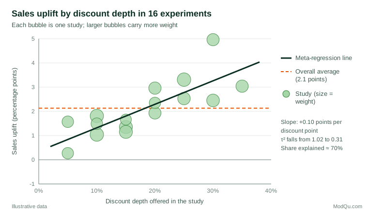
Note what the analysis does not show. It does not prove that deeper discounts cause larger uplifts. Studies with deeper discounts may also have run in different seasons, used different customer lists or promoted different products. Discount depth was not randomised across studies, so the slope is an observational association between study characteristics and results.
Categorical moderators and subgroups
Moderators need not be numeric. A categorical characteristic, such as whether a survey was run online or by telephone, enters the model as one or more dummy variables, exactly as in ordinary regression. With a single categorical moderator, meta-regression is closely related to a subgroup analysis that compares pooled estimates between groups of studies. The regression form has two advantages: it tests the difference between groups directly rather than comparing two separate intervals, and it can adjust for several characteristics at once (Borenstein et al., 2009). Continuous moderators, such as sample size, year of fieldwork or price level, can be added in the same way, and a regression on a study's standard error is a familiar check for small-study effects. Interactions between moderators are possible in principle but are rarely estimable with the small number of studies typical in practice.
Practical guidance for business and survey data
- Pre-specify a short list of moderators. Choose covariates from theory or business logic before looking at the results. Thompson and Higgins (2002) recommend this as the single most important safeguard.
- Respect the number of studies. Meta-regression has as many "observations" as studies, not respondents. With 10 or 15 studies, one or two moderators is the practical limit.
- Control false positives. Testing many candidate moderators inflates the chance of a spurious finding. Higgins and Thompson (2004) show how high this rate can be and suggest permutation tests to keep it in check.
- Use random-effects estimation and good software. The metafor package for R implements random-effects meta-regression, several τ² estimators and the Knapp–Hartung adjustment (Viechtbauer, 2010).
- Report both overall and moderated results. Give the pooled average, τ², I², the moderator coefficients with intervals and the residual heterogeneity, and show a bubble plot.
Meta-regression has long been used beyond medicine. In economics, Stanley and Jarrell (1989) proposed it as a quantitative method of reviewing literatures, for example to explain why published elasticities differ with data source and model specification. The same logic applies to a company's own archive of tracking waves, concept tests or advertising experiments.
Common mistakes
- The ecological fallacy. A study-level association need not hold for individuals. If studies with older samples show smaller effects, that does not prove the effect is smaller for older people; it may reflect other features of those studies. Berlin et al. (2002) showed that study-level meta-regression can miss an effect modifier that individual-level data reveal clearly.
- Treating a moderator as a cause. Study characteristics are not randomly assigned, so moderators are often confounded with each other.
- Using a fixed-effect meta-regression when residual heterogeneity is present, which overstates precision (Thompson & Sharp, 1999).
- Fishing for moderators after seeing the data, then reporting only the one that "worked".
- Ignoring dependence. Several effect sizes from the same study or the same customer panel are not independent and need multilevel or robust methods.
- Extrapolating. A slope estimated over discounts of 5% to 35% says nothing reliable about a 60% discount.
Key takeaways
Meta-regression turns the question "do the studies disagree?" into "what explains the disagreement?" It models effect sizes as a function of study-level covariates, weights studies by their precision plus residual heterogeneity, and reports how much of the between-study variance each moderator explains. Used with a random-effects model, a short pre-specified list of moderators and honest reporting, it is a powerful way to learn from a body of evidence. Its findings remain observational associations across studies, and they should be presented as hypotheses to test rather than as proof of cause.
References
Berkey, C. S., Hoaglin, D. C., Mosteller, F., & Colditz, G. A. (1995). A random-effects regression model for meta-analysis. Statistics in Medicine, 14(4), 395–411. https://doi.org/10.1002/sim.4780140406
Berlin, J. A., Santanna, J., Schmid, C. H., Szczech, L. A., & Feldman, H. I. (2002). Individual patient- versus group-level data meta-regressions for the investigation of treatment effect modifiers: Ecological bias rears its ugly head. Statistics in Medicine, 21(3), 371–387. https://doi.org/10.1002/sim.1023
Borenstein, M., Hedges, L. V., Higgins, J. P. T., & Rothstein, H. R. (2009). Introduction to meta-analysis. Wiley. https://doi.org/10.1002/9780470743386
DerSimonian, R., & Laird, N. (1986). Meta-analysis in clinical trials. Controlled Clinical Trials, 7(3), 177–188. https://doi.org/10.1016/0197-2456(86)90046-2
Glass, G. V. (1976). Primary, secondary, and meta-analysis of research. Educational Researcher, 5(10), 3–8. https://doi.org/10.3102/0013189X005010003
Higgins, J. P. T., & Thompson, S. G. (2002). Quantifying heterogeneity in a meta-analysis. Statistics in Medicine, 21(11), 1539–1558. https://doi.org/10.1002/sim.1186
Higgins, J. P. T., & Thompson, S. G. (2004). Controlling the risk of spurious findings from meta-regression. Statistics in Medicine, 23(11), 1663–1682. https://doi.org/10.1002/sim.1752
Knapp, G., & Hartung, J. (2003). Improved tests for a random effects meta-regression with a single covariate. Statistics in Medicine, 22(17), 2693–2710. https://doi.org/10.1002/sim.1482
Stanley, T. D., & Jarrell, S. B. (1989). Meta-regression analysis: A quantitative method of literature surveys. Journal of Economic Surveys, 3(2), 161–170. https://doi.org/10.1111/j.1467-6419.1989.tb00064.x
Thompson, S. G., & Higgins, J. P. T. (2002). How should meta-regression analyses be undertaken and interpreted? Statistics in Medicine, 21(11), 1559–1573. https://doi.org/10.1002/sim.1187
Thompson, S. G., & Sharp, S. J. (1999). Explaining heterogeneity in meta-analysis: A comparison of methods. Statistics in Medicine, 18(20), 2693–2708. https://doi.org/10.1002/(SICI)1097-0258(19991030)18:20<2693::AID-SIM235>3.0.CO;2-V
Viechtbauer, W. (2010). Conducting meta-analyses in R with the metafor package. Journal of Statistical Software, 36(3), 1–48. https://doi.org/10.18637/jss.v036.i03