
Statistics · Tests and models
Change-Point Detection Methods for Identifying Shifts in Knowledge Processes
How change-point methods find the moments when a tracking score, sales series or process measure shifts, how offline and online approaches differ, and how to avoid mistaking noise for change.
Business data rarely stay still. A brand's satisfaction score drops after a product recall, weekly complaints rise after a change of supplier, conversion rates jump after a website redesign and survey estimates shift when the fieldwork mode changes. Sometimes the timing of these shifts is known in advance. Often it is not, and the first question is simply: did something change, and if so, when?
Change-point detection is the family of statistical methods built to answer that question. A change point is a moment at which the statistical properties of a sequence, such as its mean, variance, trend or correlation structure, change abruptly. Change-point methods estimate how many such moments there are, where they occur and how large the shifts are, while allowing for the ordinary noise that makes every series wobble (Truong et al., 2020; Aminikhanghahi & Cook, 2017).
What counts as a change
A change-point model divides a series into segments, each with its own stable behaviour. The simplest and most common case is a change in mean: the series fluctuates around one level, then jumps to another. Other changes matter too:
- Change in variance, such as a sales series that becomes more volatile after entering a new market.
- Change in trend or regression relationship, such as a weakening link between advertising spend and enquiries.
- Change in distribution, where the shape of responses changes, for example when a rating scale starts to show more extreme answers.
Formally, with observations y1, …, yn and m change points at positions τ1 < τ2 < … < τm, the series is split into m + 1 segments, and the data within each segment are assumed to come from one stable distribution. The task is to estimate m and the positions τj.
Offline and online detection
Two different settings call for different methods.
Offline (retrospective) detection looks at a complete series after the fact and asks where the changes were. It is used to clean historical data, to split a tracking study into comparable periods or to explain what happened during a past year. Because all the data are available, offline methods can use observations on both sides of a candidate change.
Online (sequential) detection processes observations as they arrive and asks whether a change has just happened. It is used for monitoring: quality control, fraud alerts, early warning on customer metrics. The goal is to raise an alarm quickly after a real change while keeping false alarms rare. This is the territory of statistical process control.
Single change points: tests and estimates
The classical starting point is a single change in the mean of independent normal observations. For each possible split point, compare the means before and after; the split that best separates the data is the estimate. Hinkley (1970) derived the maximum likelihood estimator of the change point in this setting and studied its sampling behaviour, showing that for a shift of fixed size the error in the estimated location does not shrink towards zero as the series gets longer, unlike most estimates.
Testing whether any change occurred is harder than it first appears. If the analyst searches over every possible split and then applies an ordinary test at the best one, the result will look significant far too often, because the search itself has been optimised for a difference. Valid tests must account for the search.
In econometrics, Chow (1960) proposed a test for a break in a regression at a known date. Andrews (1993) extended this to an unknown date by taking the largest test statistic over a range of candidate dates and providing the correct critical values for that maximum. These tests are standard for detecting structural breaks in economic relationships.
For data that are not normally distributed, rank-based tests avoid strong assumptions. Pettitt (1979) proposed a nonparametric test based on ranks, closely related to the Mann–Whitney test, that is widely used for detecting a single shift in environmental and hydrological records and works equally well for skewed business series.
Multiple change points: search methods
Real series often contain several changes. Three ingredients define most multiple change-point methods (Truong et al., 2020): a cost function that measures how well a segment is described by a single stable model, a search method that explores possible segmentations, and a penalty or constraint that stops the method from adding too many change points.
The penalised cost
The most common formulation chooses the segmentation that minimises:
Σj C(y(τj−1+1):τj) + β·m
where C is the cost of each segment, often twice the negative log-likelihood, and β is a penalty for each additional change point. A small penalty finds many changes; a large one finds few. Penalties based on information criteria, such as the Bayesian information criterion, are common defaults, but the choice should be checked against the purpose of the analysis.
Binary segmentation
Binary segmentation applies a single change-point method to the whole series, splits at the best point if the change is significant, and then repeats the process on each part. The idea goes back to Scott and Knott (1974), who used a similar splitting rule to group treatment means in analysis of variance. Binary segmentation is fast and easy to understand, but it can miss changes that are close together or that partly cancel each other out, because the first split is chosen while ignoring later ones.
Wild binary segmentation (Fryzlewicz, 2014) fixes much of this weakness by searching many randomly drawn sub-intervals of the series, so that each change is likely to be examined in an interval where it stands alone. It keeps most of the speed of binary segmentation while improving accuracy.
Exact methods: dynamic programming and PELT
Dynamic programming finds the segmentation that exactly minimises the penalised cost. Bai and Perron (1998) developed estimation and testing for multiple structural changes in linear regression models, and Bai and Perron (2003) showed how to compute the optimal break dates efficiently with dynamic programming, together with practical advice on testing for the number of breaks.
Exact search used to be slow for long series, since the cost rises with the square of the length. Killick et al. (2012) introduced PELT (Pruned Exact Linear Time), which discards candidate change points that can never be optimal. PELT returns the same answer as full optimal partitioning but, under mild conditions such as the number of changes growing with the length of the series, its computing cost grows only linearly. It has become a default choice for offline detection. Killick and Eckley (2014) describe a widely used open-source implementation.
Nonparametric and multivariate methods
When the changes may affect the whole distribution, or several series at once, nonparametric methods are useful. Matteson and James (2014) proposed the E-divisive method, which uses energy distances between groups of observations to detect changes in any aspect of a multivariate distribution, without assuming a particular model. It suits panels where several indicators are tracked together.
Bayesian approaches
Bayesian change-point models treat the number and location of changes as unknown quantities with prior distributions and report posterior probabilities. Barry and Hartigan (1993) developed a product partition model that gives, for each time point, the posterior probability that a change occurs there. Adams and MacKay (2007) proposed Bayesian online change-point detection, which updates, as each observation arrives, the probability distribution of the "run length", the time since the most recent change.
Online detection: CUSUM and related charts
The cumulative sum (CUSUM) procedure introduced by Page (1954) is the classic online method. To detect a drop in the mean below a baseline μ0, it accumulates evidence week by week:
St = max(0, St−1 + (μ0 − k) − yt), with S0 = 0
The reference value k, often set at half the size of the shift worth detecting, stops ordinary noise from building up. When St exceeds a decision limit h, an alarm is raised. Because CUSUM accumulates small, consistent departures, it detects modest persistent shifts much faster than charts that look at one observation at a time.
The exponentially weighted moving average (EWMA) chart (Roberts, 1959) is a close alternative. It tracks a weighted average in which recent observations count more, and it is also sensitive to small sustained shifts. Both charts are central tools of statistical process control and translate naturally from manufacturing to service metrics.
The key design trade-off for online methods is between the average run length to a false alarm when nothing has changed and the detection delay when a real change occurs. Raising h reduces false alarms but slows detection. Setting these values should reflect the cost of each kind of error: a missed drop in customer satisfaction may cost more than an unnecessary investigation.
A worked example
A hypothetical company tracks its Net Promoter Score weekly from a continuous customer survey. Over two years (104 weeks) the score fluctuates by a few points from week to week because of sampling noise. The analytics team suspects that a change in the service model hurt the score for a period and wants to know when it happened and whether the score has recovered.
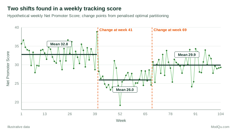
Offline analysis. Applying exact penalised optimal partitioning for changes in mean, with a cost based on the normal likelihood and a penalty of the Bayesian information criterion type, finds two change points (Figure 1). The score averages 32.8 in weeks 1 to 40, falls to 26.0 in weeks 41 to 68 and recovers to 29.9 from week 69 onwards. In this simulated series the true changes were at weeks 41 and 71, so the method finds the first exactly and places the second two weeks early, which is typical: locations are estimated with some error, especially when the shift is small relative to the noise. The analysis also gives a clear answer to the business question: the score has recovered part of the way, but not to its earlier level.
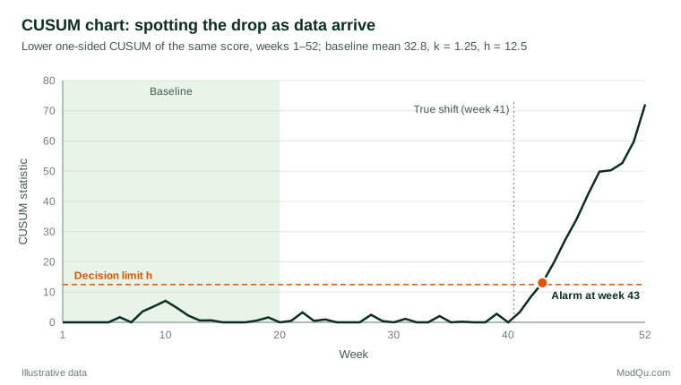
Online analysis. Suppose instead that the team had been monitoring the score live. Using the first 20 weeks as a baseline (mean 32.8, with the week-to-week standard deviation taken as 2.5), it runs a lower one-sided CUSUM with k = 1.25 and h = 12.5, that is, half a standard deviation and five standard deviations (Figure 2). The statistic rises occasionally during the stable period but never approaches the limit. After the shift at week 41 it climbs steeply and crosses the limit at week 43, two weeks after the change. A simple chart that flags single weeks more than three standard deviations below the baseline would have signalled at week 44 here, because this drop is large. For smaller shifts the advantage of CUSUM grows, since no single week may ever cross a three-standard-deviation limit while the accumulated evidence still does.
Change points and intervention analysis
When the date of a possible change is known, such as a price rise or a campaign launch, the question becomes one of intervention analysis rather than detection. Box and Tiao (1975) set out models for estimating the effect of an intervention on a time series while accounting for autocorrelation. Segmented regression of interrupted time series estimates changes in both level and trend at a known date (Wagner et al., 2002), and Lopez Bernal et al. (2017) give a practical tutorial covering design, seasonality and common pitfalls.
The two approaches complement each other. Change-point detection can confirm whether the largest shift in a series actually occurred at the date of the intervention or somewhere else, which is a useful check against attributing a change to the wrong cause.
Applications in survey and business data
- Tracking studies. Detect shifts in brand awareness, satisfaction or purchase intent, and split long series into periods with stable levels for reporting.
- Methodology changes. Changes of survey mode, questionnaire wording, sample supplier or weighting scheme can create artificial jumps. Climate scientists face the same problem when instruments or station locations change; Reeves et al. (2007) reviewed and compared change-point techniques for finding such undocumented shifts, and the lessons transfer directly to survey time series.
- Operational monitoring. CUSUM and EWMA charts on complaint rates, response rates, delivery times and fraud indicators give early warning with controlled false-alarm rates.
- Economic and market analysis. Structural break tests check whether relationships, such as price elasticity or the link between confidence and spending, have changed. Zeileis et al. (2002) describe freely available software for testing and dating structural changes in regression models.
Practical guidance
- Define the change of interest. Decide whether you are looking for shifts in level, variance, trend or distribution, and choose a cost function to match. A method for changes in mean will not reliably detect a change in variance.
- Account for autocorrelation and seasonality. Most basic methods assume independent observations. Positive autocorrelation makes ordinary wandering look like shifts and leads to too many change points. Model seasonality and autocorrelation first, or use methods that allow for them.
- Choose the penalty deliberately. The number of change points depends heavily on the penalty. Plot results across a range of penalties and prefer segmentations that remain stable.
- Report uncertainty in locations. A change point is an estimate. Report a range of plausible dates or posterior probabilities where possible, especially before linking a change to a specific event.
- Check sample sizes behind each point. In survey tracking, weekly estimates based on small samples are noisy. Use effective sample sizes after weighting to set expectations for the size of shift that can be detected.
- Use tested software. Mature, openly documented implementations exist for PELT, binary segmentation, structural break tests and CUSUM charts (Killick & Eckley, 2014; Zeileis et al., 2002).
- Separate detection from explanation. Detection says when something changed. Explanation requires additional evidence: timelines of events, segment-level analysis and, ideally, a comparison series that was not affected.
Limitations and common mistakes
- Mistaking noise for change. Searching for the best split always finds one. Without a valid test or penalty, random fluctuations will be reported as shifts.
- Ignoring multiple testing in monitoring. Running many control charts at once across products, regions and metrics raises the overall chance of false alarms. Adjust limits or use methods that control the false discovery rate across charts.
- Assuming abrupt change. Some processes drift gradually. Forcing a step model onto a slow trend produces a staircase of spurious change points. Compare change-point models with smooth trend models.
- Confusing coincidence with cause. A change that coincides with a campaign or a policy may have other causes. Change-point analysis identifies when, not why.
Key takeaways
Change-point detection finds the moments when a process stops behaving as it did before. Offline methods such as binary segmentation, wild binary segmentation, dynamic programming and PELT divide a completed series into stable segments, while online methods such as CUSUM and EWMA raise alarms soon after a change as data arrive. Good practice means defining the type of change of interest, allowing for autocorrelation and seasonality, choosing penalties and alarm limits deliberately and reporting uncertainty about where changes occurred. Used this way, they turn noisy tracking data into a defensible account of when things changed.
References
Adams, R. P., & MacKay, D. J. C. (2007). Bayesian online changepoint detection (arXiv:0710.3742). arXiv. https://doi.org/10.48550/arXiv.0710.3742
Aminikhanghahi, S., & Cook, D. J. (2017). A survey of methods for time series change point detection. Knowledge and Information Systems, 51(2), 339–367. https://doi.org/10.1007/s10115-016-0987-z
Andrews, D. W. K. (1993). Tests for parameter instability and structural change with unknown change point. Econometrica, 61(4), 821–856. https://doi.org/10.2307/2951764
Bai, J., & Perron, P. (1998). Estimating and testing linear models with multiple structural changes. Econometrica, 66(1), 47–78. https://doi.org/10.2307/2998540
Bai, J., & Perron, P. (2003). Computation and analysis of multiple structural change models. Journal of Applied Econometrics, 18(1), 1–22. https://doi.org/10.1002/jae.659
Barry, D., & Hartigan, J. A. (1993). A Bayesian analysis for change point problems. Journal of the American Statistical Association, 88(421), 309–319. https://doi.org/10.1080/01621459.1993.10594323
Box, G. E. P., & Tiao, G. C. (1975). Intervention analysis with applications to economic and environmental problems. Journal of the American Statistical Association, 70(349), 70–79. https://doi.org/10.1080/01621459.1975.10480264
Chow, G. C. (1960). Tests of equality between sets of coefficients in two linear regressions. Econometrica, 28(3), 591–605. https://doi.org/10.2307/1910133
Fryzlewicz, P. (2014). Wild binary segmentation for multiple change-point detection. The Annals of Statistics, 42(6), 2243–2281. https://doi.org/10.1214/14-AOS1245
Hinkley, D. V. (1970). Inference about the change-point in a sequence of random variables. Biometrika, 57(1), 1–17. https://doi.org/10.1093/biomet/57.1.1
Killick, R., & Eckley, I. A. (2014). changepoint: An R package for changepoint analysis. Journal of Statistical Software, 58(3), 1–19. https://doi.org/10.18637/jss.v058.i03
Killick, R., Fearnhead, P., & Eckley, I. A. (2012). Optimal detection of changepoints with a linear computational cost. Journal of the American Statistical Association, 107(500), 1590–1598. https://doi.org/10.1080/01621459.2012.737745
Lopez Bernal, J., Cummins, S., & Gasparrini, A. (2017). Interrupted time series regression for the evaluation of public health interventions: A tutorial. International Journal of Epidemiology, 46(1), 348–355. https://doi.org/10.1093/ije/dyw098
Matteson, D. S., & James, N. A. (2014). A nonparametric approach for multiple change point analysis of multivariate data. Journal of the American Statistical Association, 109(505), 334–345. https://doi.org/10.1080/01621459.2013.849605
Page, E. S. (1954). Continuous inspection schemes. Biometrika, 41(1–2), 100–115. https://doi.org/10.1093/biomet/41.1-2.100
Pettitt, A. N. (1979). A non-parametric approach to the change-point problem. Journal of the Royal Statistical Society Series C: Applied Statistics, 28(2), 126–135. https://doi.org/10.2307/2346729
Reeves, J., Chen, J., Wang, X. L., Lund, R., & Lu, Q. Q. (2007). A review and comparison of changepoint detection techniques for climate data. Journal of Applied Meteorology and Climatology, 46(6), 900–915. https://doi.org/10.1175/JAM2493.1
Roberts, S. W. (1959). Control chart tests based on geometric moving averages. Technometrics, 1(3), 239–250. https://doi.org/10.1080/00401706.1959.10489860
Scott, A. J., & Knott, M. (1974). A cluster analysis method for grouping means in the analysis of variance. Biometrics, 30(3), 507–512. https://doi.org/10.2307/2529204
Truong, C., Oudre, L., & Vayatis, N. (2020). Selective review of offline change point detection methods. Signal Processing, 167, Article 107299. https://doi.org/10.1016/j.sigpro.2019.107299
Wagner, A. K., Soumerai, S. B., Zhang, F., & Ross-Degnan, D. (2002). Segmented regression analysis of interrupted time series studies in medication use research. Journal of Clinical Pharmacy and Therapeutics, 27(4), 299–309. https://doi.org/10.1046/j.1365-2710.2002.00430.x
Zeileis, A., Leisch, F., Hornik, K., & Kleiber, C. (2002). strucchange: An R package for testing for structural change in linear regression models. Journal of Statistical Software, 7(2), 1–38. https://doi.org/10.18637/jss.v007.i02