
Statistics · Tests and models
Copula Methods for Modeling Dependence Structures in Multivariate Knowledge
How copulas separate the behaviour of each variable from the way variables move together, why a single correlation can hide joint extremes, and how to use copulas with survey and business data.
Many business risks and opportunities depend less on any one variable than on how several variables move together. A retailer cares whether demand for two products peaks in the same week. An insurer cares whether storm claims and flood claims arrive together. A customer experience team cares whether the customers who are least satisfied are also the ones most likely to leave. In each case the question is about dependence, and especially about what happens in the extremes.
The usual summary of dependence, a single correlation coefficient, answers that question poorly. Copulas offer a more complete answer. A copula is a function that describes how variables are linked, separately from the distribution of each variable on its own. That separation lets analysts model skewed spending, bounded scores and heavy-tailed losses with whatever distributions fit them best, and then choose a dependence structure that matches how the variables really behave together, including in the tails (Nelsen, 2006; Joe, 2014).
This article explains the idea behind copulas, introduces the main families, works through an example and gives practical guidance for survey, market research and business data.
Why correlation is not enough
Pearson's correlation coefficient measures linear association. It is a complete description of dependence only in special cases, most notably when variables follow a joint normal distribution. Embrechts et al. (2002) set out the pitfalls of relying on it outside that setting. Correlation changes when the variables are transformed, for example from spend to log spend, even though the underlying relationship is the same. Two pairs of variables can share the same margins and the same correlation yet behave very differently when one of them is extreme. And for some pairs of margins, not every correlation between −1 and 1 is even possible.
Rank-based measures avoid part of the problem. Kendall's tau (Kendall, 1938) and Spearman's rho depend only on the ordering of the observations, so they do not change when a variable is stretched or compressed by a monotonic transformation. But a single number, however robust, still cannot say whether the association is concentrated among low values, high values or spread evenly. For risk, retention and demand planning, that distinction often matters most.
Sklar's theorem: separating margins from dependence
The theoretical foundation of copula modelling is a result published by Sklar (1959). For two continuous variables X and Y with distribution functions F and G, their joint distribution H can always be written as:
H(x, y) = C(F(x), G(y))
Here C is the copula: a joint distribution function on the unit square whose margins are uniform between 0 and 1. If the margins are continuous, the copula is unique. The theorem works in both directions. Any copula combined with any margins gives a valid joint distribution, and any joint distribution contains a copula that can be extracted from it.
The intuition is simple. Applying a variable's own distribution function, U = F(X), turns each observation into its percentile rank. The copula is the joint distribution of those ranks. It contains all the information about how the variables are associated and nothing about their scales, units or shapes. Genest and MacKay (1986) gave an accessible early introduction to the idea for statisticians, describing copulas as bivariate distributions with uniform margins, and the concept now underpins much of modern dependence modelling (Joe, 2014).
This separation has three practical benefits:
- Flexible margins. One variable can be modelled with a gamma distribution, another with a beta or an empirical distribution, without forcing either into a normal shape.
- Scale-free dependence. Rank-based dependence measures such as Kendall's tau are functions of the copula alone, so they are unaffected by how each variable is measured.
- Modular modelling. Analysts can change the dependence structure while leaving the margins untouched, which makes it easy to test how sensitive a conclusion is to assumptions about joint behaviour.
Main copula families
Hundreds of copulas have been proposed, but a few families do most of the work in applied statistics. Nelsen (2006) and Joe (2014) provide comprehensive catalogues.
Elliptical copulas
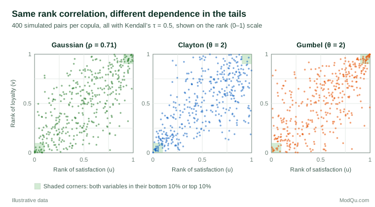
The Gaussian copula is the dependence structure of a multivariate normal distribution, applied to any margins. It is defined by a correlation matrix and is easy to use in many dimensions. Its weakness is that it has no tail dependence: as one goes further into the extremes, the chance that the other variable is also extreme fades away, however strong the correlation. The t copula adds a degrees-of-freedom parameter that creates symmetric tail dependence, so joint extremes in both directions are more likely (McNeil et al., 2015).
Archimedean copulas
Archimedean copulas are built from a single generator function and usually have one parameter, θ. Three are especially common:
- The Clayton copula (Clayton, 1978), originally developed for associations in family disease histories, has dependence concentrated in the lower tail.
- The Gumbel copula (Gumbel, 1960) has dependence concentrated in the upper tail.
- The Frank copula (Frank, 1979) is symmetric and has no tail dependence.
For the bivariate Clayton copula the formula is:
C(u, v) = (u−θ + v−θ − 1)−1/θ, θ > 0
and for the Gumbel copula:
C(u, v) = exp(−[(−ln u)θ + (−ln v)θ]1/θ), θ ≥ 1
Each parameter has a simple link to Kendall's tau. For Clayton, τ = θ ÷ (θ + 2); for Gumbel, τ = 1 − 1/θ; for the Gaussian copula, the correlation parameter is ρ = sin(πτ ÷ 2) (Nelsen, 2006). These relationships make it easy to compare families on a common footing.
Rotations and negative dependence
Archimedean families are not limited to one corner. Rotating a copula by 180 degrees gives its survival copula, so a rotated Clayton copula has upper-tail rather than lower-tail dependence. Rotations by 90 or 270 degrees turn positive dependence into negative dependence, which is useful for pairs such as price and purchase volume, where high values of one tend to accompany low values of the other (Joe, 2014). Rotations greatly extend the range of patterns a small set of families can represent.
Tail dependence
The coefficient of tail dependence measures the limiting probability that one variable is extreme given that the other is equally extreme. For Clayton the lower-tail coefficient is 2−1/θ; for Gumbel the upper-tail coefficient is 2 − 21/θ; for the Gaussian copula both are zero whenever the correlation is below 1. With θ = 2, Clayton has a lower-tail coefficient of about 0.71 and Gumbel an upper-tail coefficient of about 0.59. These numbers matter whenever the business question concerns the corners of the distribution: simultaneous losses, simultaneous stock-outs or customers who are extreme on several warning signs at once.
Fitting copulas to data
Copula models are usually fitted in two stages, which keeps the work manageable.
Stage 1: model or rank the margins. Each variable is converted to the unit interval. In the parametric approach, a distribution is fitted to each variable and its fitted distribution function is applied. The inference functions for margins method then estimates the copula parameters with the fitted margins held fixed (Joe, 2014). In the semiparametric approach, each observation is simply replaced by its rank divided by n + 1, giving pseudo-observations. Genest et al. (1995) showed that maximising the copula likelihood on these pseudo-observations gives consistent and asymptotically normal estimates, without any assumption about the margins. This rank-based route is usually the safer choice when the margins are hard to model.
Stage 2: estimate the copula. Parameters can be estimated by maximum likelihood on the transformed data or, more simply, by inverting Kendall's tau: compute the sample tau and solve the family's formula for θ. Genest and Favre (2007) give a clear step-by-step tutorial, with a worked hydrological example, covering rank plots, moment-type estimators, pseudo-likelihood and model checking.
Model checking. Different families with the same tau can fit very differently in the tails, so the choice of family must be checked. Genest et al. (2009) reviewed goodness-of-fit tests for copulas and compared their power in a large simulation study; tests based on the empirical copula process performed well across many settings. Information criteria, plots of the pseudo-observations and comparisons of empirical and fitted tail probabilities complement formal tests.
Mature open-source software implements these steps. Hofert et al. (2018) describe estimation, simulation and goodness-of-fit testing for a wide range of families using freely available tools, which reduces the risk of errors in hand-written code.
Beyond two variables: vine copulas
Most business problems involve more than two variables. Multivariate Gaussian and t copulas scale easily but impose the same type of dependence on every pair. Multivariate Archimedean copulas are even more restrictive, because a single parameter governs all pairs.
Vine copulas, also called pair-copula constructions, solve this by building a high-dimensional dependence structure from a cascade of bivariate copulas. Bedford and Cooke (2002) introduced vines as graphical models for dependent variables, and Aas et al. (2009) showed how to estimate pair-copula constructions in practice, illustrating them on financial return data. Each pair, or conditional pair, can use a different family, so one link might have strong lower-tail dependence while another is symmetric. Czado (2019) provides a practical guide to selecting the vine structure, choosing pair families and fitting the model.
Vines are powerful but demanding. The number of possible structures grows very quickly with the number of variables, so automated selection, simplifying assumptions and careful validation are needed.
Dependence over time
Copulas also apply to time series. Patton (2006) introduced conditional copulas, in which the dependence parameter can change over time with past observations, and used them to show that dependence between exchange rates was asymmetric and time-varying. Patton (2012) later reviewed copula models for economic time series, covering estimation, inference and forecasting. The usual approach is to model each series with its own time-series model, such as an autoregressive model with time-varying volatility, and then link the standardised residuals with a copula.
A worked example
A hypothetical subscription business runs a customer survey and links it to account records. Two variables interest the retention team: a satisfaction index and a loyalty index built from renewal intent and usage. Both are skewed, and the sample Kendall's tau between them is 0.5.
The team wants to know how many customers are in the bottom 10% on both measures at once. These customers are the most likely to cancel and the natural first target for outreach. If the two variables were independent, the answer would be 10% × 10% = 1% of customers. With positive dependence it is clearly higher, but how much higher depends on the copula.
Using the formulas above, with each family calibrated to τ = 0.5:
| Dependence model | Both in bottom 10% | Both in top 10% | Share of bottom-10% satisfaction who are also bottom-10% loyalty |
|---|---|---|---|
| Independence | 1.0% | 1.0% | 10% |
| Gaussian (ρ = 0.71) | 4.7% | 4.7% | 47% |
| Clayton (θ = 2) | 7.1% | 2.5% | 71% |
| Gumbel (θ = 2) | 3.9% | 6.2% | 39% |
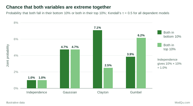
For a hypothetical base of 100,000 customers, the Gaussian copula implies about 4,700 customers in the at-risk corner, while the Clayton copula implies about 7,100: a difference of roughly 2,400 customers, or half as many again, from the same tau. If dissatisfaction and disloyalty tend to go together more strongly at the bottom of the scale than at the top, which is plausible when a single bad experience drives both, the Gaussian assumption understates the at-risk group and the retention budget will be set too low.
Which model is right is an empirical question. The team would plot the pseudo-observations, compare empirical counts in each corner with the fitted values, run a goodness-of-fit test and check the result on a holdout wave. The point of the example is that the choice of copula is a substantive business assumption, not a technical detail.
Applications in business and market research
- Finance and insurance. Copulas are standard tools for aggregating risks, pricing portfolios of credit exposures and modelling joint claims (McNeil et al., 2015). Li (2000) introduced the Gaussian copula approach to default correlation that became widely used in pricing collateralised debt obligations.
- Marketing. Danaher and Smith (2011) showed how copulas can build multivariate models for marketing data whose margins are discrete, skewed or otherwise non-normal, and demonstrated gains over approaches that force a multivariate normal shape.
- Econometrics. Trivedi and Zimmer (2007) introduced copulas to applied economists, covering estimation, model selection and applications with mixed continuous and discrete outcomes.
- Simulation and synthetic data. Because a copula can be sampled and then combined with any margins, it is a convenient way to create realistic joint scenarios for stress tests, demand planning and Monte Carlo simulation of multiple linked inputs.
- Survey data fusion. When variables from different sources must be linked, a copula fitted on a sample that contains both variables can generate joint distributions that respect each source's own margins.
Practical guidance for survey and business data
- Start with rank plots. Plot the pseudo-observations for each pair. Clustering in one corner is the first sign that a symmetric model is inadequate.
- Use rank-based estimation when margins are uncertain. Pseudo-likelihood avoids errors in the margins spilling into the dependence estimate.
- Fit several families and compare tails. Report how sensitive the key quantity, such as the size of an at-risk group, is to the choice of copula. If the conclusion changes, say so.
- Be careful with discrete data. Likert items, counts and yes/no outcomes have ties, and with discrete margins the copula is no longer unique. Rank-based methods designed for continuous data can mislead in that case; specialised methods are needed (Joe, 2014; Trivedi & Zimmer, 2007).
- Respect the sample design. Use survey weights when computing empirical distribution functions and dependence measures from weighted samples, and use resampling methods that reflect the design for standard errors.
- Check stability over time. Dependence often strengthens during crises or market shocks. Fitting a single copula to a long period can average together very different regimes (Patton, 2012).
Communicating results to decision-makers
Copula parameters such as θ mean little to most audiences. Translate the fitted model into quantities that answer the business question: the expected number of customers who fall into a risk corner, the probability that two regions both miss their sales targets in the same quarter, or the chance that two cost lines both exceed budget. Show how these quantities change across plausible copula families, so that readers see the uncertainty that comes from the dependence assumption as well as from sampling. Simple visual tools work well: scatter plots of percentile ranks, tables of joint exceedance probabilities and side-by-side comparisons like Figure 2. Where a decision depends heavily on the tail, present a range rather than a single figure.
Limitations and common mistakes
Copulas are tools, not answers. Several mistakes recur in practice.
- Treating the Gaussian copula as neutral. It is often chosen because it is familiar, but it rules out tail dependence by construction. MacKenzie and Spears (2014) document how the Gaussian copula became embedded in investment banking practice before the 2007–2008 crisis, and how its limitations in modelling joint defaults were understood but often set aside.
- Overfitting. Flexible families and vines can fit a sample very closely while generalising poorly. Use holdout data and information criteria.
- Small samples in the tails. Tail dependence is, by definition, estimated from few observations. Confidence intervals for tail quantities are often wide and should be reported.
- Expecting copulas to explain causes. A copula describes association. It does not say why variables move together or what would happen if one were changed.
- Uncritical enthusiasm. Mikosch (2006) argued that copulas had been promoted beyond what their theory supports, especially in time series and extreme-value settings, and that the separation of margins and dependence is less clean than it appears when the margins are unknown. His critique, and the responses to it, are a useful corrective for any team adopting copulas.
Key takeaways
Copulas separate two questions that a single correlation mixes together: how each variable is distributed and how variables move together. Sklar's theorem guarantees that any joint distribution can be split in this way. Families such as Gaussian, t, Clayton, Gumbel and Frank offer different patterns of dependence, and vines extend them to many variables. Two models with the same rank correlation can give very different answers about joint extremes, as the worked example shows, so choosing a copula is a substantive decision that should be checked against data. Used with care, copulas give survey analysts, risk managers and planners a more honest picture of how outcomes cluster together, especially in the corners where the biggest risks and opportunities lie.
References
Aas, K., Czado, C., Frigessi, A., & Bakken, H. (2009). Pair-copula constructions of multiple dependence. Insurance: Mathematics and Economics, 44(2), 182–198. https://doi.org/10.1016/j.insmatheco.2007.02.001
Bedford, T., & Cooke, R. M. (2002). Vines: A new graphical model for dependent random variables. The Annals of Statistics, 30(4), 1031–1068. https://doi.org/10.1214/aos/1031689016
Clayton, D. G. (1978). A model for association in bivariate life tables and its application in epidemiological studies of familial tendency in chronic disease incidence. Biometrika, 65(1), 141–151. https://doi.org/10.1093/biomet/65.1.141
Czado, C. (2019). Analyzing dependent data with vine copulas: A practical guide with R. Springer. https://doi.org/10.1007/978-3-030-13785-4
Danaher, P. J., & Smith, M. S. (2011). Modeling multivariate distributions using copulas: Applications in marketing. Marketing Science, 30(1), 4–21. https://doi.org/10.1287/mksc.1090.0491
Embrechts, P., McNeil, A. J., & Straumann, D. (2002). Correlation and dependence in risk management: Properties and pitfalls. In M. A. H. Dempster (Ed.), Risk management: Value at risk and beyond (pp. 176–223). Cambridge University Press. https://doi.org/10.1017/CBO9780511615337.008
Frank, M. J. (1979). On the simultaneous associativity of F(x, y) and x + y − F(x, y). Aequationes Mathematicae, 19(1), 194–226. https://doi.org/10.1007/BF02189866
Genest, C., & Favre, A.-C. (2007). Everything you always wanted to know about copula modeling but were afraid to ask. Journal of Hydrologic Engineering, 12(4), 347–368. https://doi.org/10.1061/(ASCE)1084-0699(2007)12:4(347)
Genest, C., Ghoudi, K., & Rivest, L.-P. (1995). A semiparametric estimation procedure of dependence parameters in multivariate families of distributions. Biometrika, 82(3), 543–552. https://doi.org/10.1093/biomet/82.3.543
Genest, C., & MacKay, J. (1986). The joy of copulas: Bivariate distributions with uniform marginals. The American Statistician, 40(4), 280–283. https://doi.org/10.1080/00031305.1986.10475414
Genest, C., Rémillard, B., & Beaudoin, D. (2009). Goodness-of-fit tests for copulas: A review and a power study. Insurance: Mathematics and Economics, 44(2), 199–213. https://doi.org/10.1016/j.insmatheco.2007.10.005
Gumbel, E. J. (1960). Bivariate exponential distributions. Journal of the American Statistical Association, 55(292), 698–707. https://doi.org/10.1080/01621459.1960.10483368
Hofert, M., Kojadinovic, I., Mächler, M., & Yan, J. (2018). Elements of copula modeling with R. Springer. https://doi.org/10.1007/978-3-319-89635-9
Joe, H. (2014). Dependence modeling with copulas. Chapman and Hall/CRC. https://doi.org/10.1201/b17116
Kendall, M. G. (1938). A new measure of rank correlation. Biometrika, 30(1–2), 81–93. https://doi.org/10.1093/biomet/30.1-2.81
Li, D. X. (2000). On default correlation: A copula function approach. The Journal of Fixed Income, 9(4), 43–54. https://doi.org/10.3905/jfi.2000.319253
MacKenzie, D., & Spears, T. (2014). "The formula that killed Wall Street": The Gaussian copula and modelling practices in investment banking. Social Studies of Science, 44(3), 393–417. https://doi.org/10.1177/0306312713517157
McNeil, A. J., Frey, R., & Embrechts, P. (2015). Quantitative risk management: Concepts, techniques and tools (Rev. ed.). Princeton University Press.
Mikosch, T. (2006). Copulas: Tales and facts. Extremes, 9(1), 3–20. https://doi.org/10.1007/s10687-006-0015-x
Nelsen, R. B. (2006). An introduction to copulas (2nd ed.). Springer. https://doi.org/10.1007/0-387-28678-0
Patton, A. J. (2006). Modelling asymmetric exchange rate dependence. International Economic Review, 47(2), 527–556. https://doi.org/10.1111/j.1468-2354.2006.00387.x
Patton, A. J. (2012). A review of copula models for economic time series. Journal of Multivariate Analysis, 110, 4–18. https://doi.org/10.1016/j.jmva.2012.02.021
Sklar, A. (1959). Fonctions de répartition à n dimensions et leurs marges. Publications de l'Institut de Statistique de l'Université de Paris, 8, 229–231.
Trivedi, P. K., & Zimmer, D. M. (2007). Copula modeling: An introduction for practitioners. Foundations and Trends in Econometrics, 1(1), 1–111. https://doi.org/10.1561/0800000005