
Statistics · Tests and models
Handling Zero-Inflated and Overdispersed Data in Count Knowledge Models
Why real counts such as visits, purchases or complaints rarely fit a Poisson model, and how negative binomial, zero-inflated and hurdle models handle extra variation and excess zeros.
Many survey and business measures are counts: store visits last month, products bought, support calls, complaints, days absent. The textbook model for counts is Poisson regression, a generalised linear model with a log link (McCullagh & Nelder, 1989). It makes a strong assumption: the variance equals the mean. Real counts almost never behave that way. They usually show overdispersion (variance larger than the mean) and often far more zeros than a Poisson model allows. Ignoring either problem produces standard errors that are too small and predictions that misrepresent who does what.
Why counts are overdispersed
Overdispersion arises whenever people differ in ways the model does not capture. Two customers with identical age, income and region may still have very different underlying visit rates. Mixing many Poisson processes with different rates produces a distribution that is more spread out than any single Poisson. Clustering (households, stores, panels) and contagion, where one purchase makes the next more likely, add to it (Cameron & Trivedi, 2013).
The consequence is not usually biased coefficients but overconfident inference. If the variance is four times the mean, Poisson standard errors are roughly half their correct size, so weak effects look significant.
Diagnosing the problem
- Compare mean and variance, overall and within groups. A variance several times the mean is a clear warning.
- Check the dispersion statistic. The Pearson chi-square divided by its residual degrees of freedom should be close to 1 for a Poisson model; values well above 1 indicate overdispersion.
- Use a formal test. Cameron and Trivedi (1990) proposed simple regression-based tests for overdispersion in the Poisson model.
- Compare observed and predicted frequencies, especially the share of zeros. This is the most intuitive check for a business audience.
Remedies for overdispersion
Quasi-Poisson keeps the Poisson mean model but scales the variance by an estimated dispersion factor, an application of the quasi-likelihood approach of Wedderburn (1974). Coefficients are unchanged and standard errors are inflated appropriately.
Negative binomial regression treats each person's rate as varying randomly around the model's prediction, which gives a variance of μ + αμ², growing with the square of the mean (Hilbe, 2011). It is a full likelihood model, so it gives predicted probabilities for every count and supports likelihood-based comparisons.
The two differ in how they weight observations. Ver Hoef and Boveng (2007) show that because quasi-Poisson variance is linear in the mean and negative binomial variance is quadratic, the two weight large and small counts differently and can give different estimates. They recommend plotting squared residuals against fitted means to see which variance pattern the data follow.
Excess zeros: two kinds of non-users
Sometimes zeros come from two different sources. In a survey on visits to a garden centre, some respondents have no garden and will never visit; others are potential customers who simply did not visit last month. The first group produces structural zeros, the second produces sampling zeros.
Zero-inflated models, introduced by Lambert (1992) for counts of defects in manufacturing, combine a binary process (is this person in the "always zero" group?) with a Poisson or negative binomial count for everyone else. Each part can have its own predictors: having a garden predicts membership of the zero group, while distance and income predict visit frequency among potential customers.
Hurdle models, proposed by Mullahy (1986), take a different view. A binary model decides whether the count is zero or positive, and a truncated count model describes how many among those who cross the hurdle. All zeros come from one process. Hurdle models suit decisions that happen in two stages, such as whether to buy at all and then how many to buy.
A worked example
A hypothetical survey of 2,000 customers asks how many times each person visited a store in the past month. The mean is 1.3 visits and the variance 3.9, three times the mean. Of the respondents, 53% made no visits.
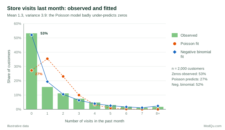
A Poisson model with the same mean predicts only 27% zeros, far too many customers with one or two visits and almost no heavy visitors. A negative binomial model predicts 52% zeros and tracks the tail closely. This illustrates an important point: many zeros do not automatically mean zero inflation. Overdispersion alone can produce a large spike at zero, and a negative binomial model may be sufficient. A zero-inflated negative binomial is worth adding when there is a substantive reason to expect a distinct never-user group and it clearly improves fit.
Choosing between models
- Start with theory. Is there a plausible group that can never record the event? If not, prefer a negative binomial or hurdle model.
- Compare fit with information criteria and observed-versus-predicted frequency tables, not only a single test.
- Be careful with the Vuong test. Vuong (1989) designed his test for non-nested models, and it is widely used to compare zero-inflated and standard models. Wilson (2015) explains that the zero-inflated Poisson model nests the standard Poisson model at a boundary, so this use of the test is invalid.
- Use software that fits all candidates. Zeileis et al. (2008) describe R functions for Poisson, negative binomial, zero-inflated and hurdle regression with a common interface.
Practical guidance for survey data
Survey counts bring their own issues. Recall over long periods produces heaping at round numbers (5, 10, 20), which no count model captures well; shorter reference periods help. Top-coded answers ("10 or more") call for censored models or careful sensitivity checks. Survey weights and clustered designs require design-based standard errors whichever count model is chosen.
Common mistakes
- Using Poisson regression without checking dispersion.
- Assuming that a large share of zeros proves zero inflation.
- Interpreting the zero-inflation part as a causal "non-user" type when it is a statistical component.
- Reporting only incidence rate ratios, without predicted counts or probabilities that decision-makers can understand.
- Ignoring exposure: counts over different time periods need an offset.
Key takeaways
Count outcomes are common in business data, and they rarely meet the Poisson assumption. Check dispersion and the share of zeros first. Use quasi-Poisson or negative binomial models for overdispersion, and add zero-inflated or hurdle components when theory points to a separate source of zeros and the data support it. Compare models on predicted frequencies as well as test statistics, and report results as predicted counts that a business reader can use.
References
Cameron, A. C., & Trivedi, P. K. (1990). Regression-based tests for overdispersion in the Poisson model. Journal of Econometrics, 46(3), 347–364. https://doi.org/10.1016/0304-4076(90)90014-K
Cameron, A. C., & Trivedi, P. K. (2013). Regression analysis of count data (2nd ed.). Cambridge University Press. https://doi.org/10.1017/CBO9781139013567
Hilbe, J. M. (2011). Negative binomial regression (2nd ed.). Cambridge University Press. https://doi.org/10.1017/CBO9780511973420
Lambert, D. (1992). Zero-inflated Poisson regression, with an application to defects in manufacturing. Technometrics, 34(1), 1–14. https://doi.org/10.2307/1269547
McCullagh, P., & Nelder, J. A. (1989). Generalized linear models (2nd ed.). Chapman and Hall. https://doi.org/10.1201/9780203753736
Mullahy, J. (1986). Specification and testing of some modified count data models. Journal of Econometrics, 33(3), 341–365. https://doi.org/10.1016/0304-4076(86)90002-3
Ver Hoef, J. M., & Boveng, P. L. (2007). Quasi-Poisson vs. negative binomial regression: How should we model overdispersed count data? Ecology, 88(11), 2766–2772. https://doi.org/10.1890/07-0043.1
Vuong, Q. H. (1989). Likelihood ratio tests for model selection and non-nested hypotheses. Econometrica, 57(2), 307–333. https://doi.org/10.2307/1912557
Wedderburn, R. W. M. (1974). Quasi-likelihood functions, generalized linear models, and the Gauss–Newton method. Biometrika, 61(3), 439–447. https://doi.org/10.1093/biomet/61.3.439
Wilson, P. (2015). The misuse of the Vuong test for non-nested models to test for zero-inflation. Economics Letters, 127, 51–53. https://doi.org/10.1016/j.econlet.2014.12.029
Zeileis, A., Kleiber, C., & Jackman, S. (2008). Regression models for count data in R. Journal of Statistical Software, 27(8), 1–25. https://doi.org/10.18637/jss.v027.i08