
Statistics · Descriptive statistics
Measures of Dispersion: Range, Variance and Standard Deviation
How the range, variance and standard deviation describe the spread of data, how to calculate and interpret them, and when robust alternatives serve survey and business data better.
An average on its own tells only half the story. Two stores can share the same mean satisfaction score while one delights almost every customer and the other splits its customers between fans and critics. Two suppliers can deliver in five days on average while one is always on time and the other is unpredictable. Measures of dispersion, also called measures of spread or variability, describe how far individual values lie from one another and from the centre of the data. They are as essential to sound reporting as the mean or the median.
This article explains the range, the variance and the standard deviation, works through an example, and sets out robust alternatives and common mistakes for survey and business data.
Why spread matters
Variation is the raw material of statistics, and spread affects almost every decision that rests on data:
- Consistency. A low average wait time is little comfort if a sizeable minority of callers wait far longer.
- Risk. In finance and operations, variability is often the very thing being managed.
- Segmentation. Wide spread in survey answers can signal distinct customer groups that an average hides.
- Precision of estimates. The more variable a population, the larger the sample needed to estimate its mean with a given margin of error (Lohr, 2021).
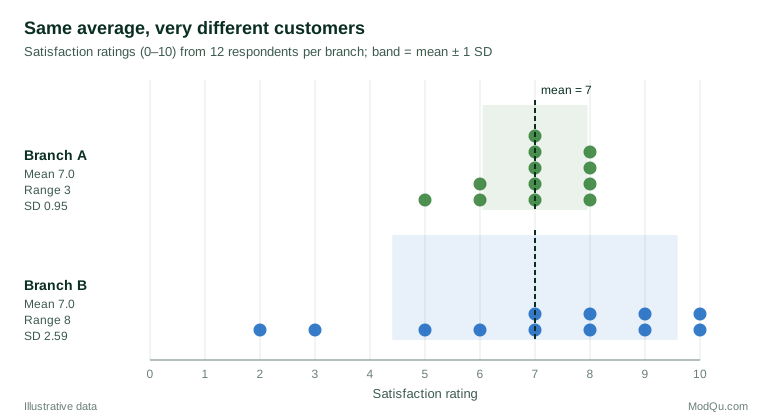
Figure 1 shows the core idea. Two hypothetical branches each receive 12 ratings with a mean of exactly 7 out of 10, yet their customers' experiences are very different.
The range
The range is the simplest measure of spread: the largest value minus the smallest.
Range = xmax − xmin
In Figure 1, Branch A's ratings run from 5 to 8, a range of 3, and Branch B's run from 2 to 10, a range of 8. It is easy to compute and explain, and the range of small samples has long been used in quality control. Tippett (1925) tabulated the expected range of samples drawn from a normal distribution, work that made it possible to convert a sample range into an estimate of the underlying standard deviation.
The range has two serious weaknesses. First, it depends on only two observations, the most extreme ones, so a single unusual value can change it dramatically. Second, it tends to grow with sample size, because larger samples are more likely to include someone at the very top or bottom of the scale. The range is best treated as a description of the observed extremes rather than of typical spread.
The interquartile range
A more stable relative of the range is the interquartile range (IQR), the distance between the first quartile (the 25th percentile) and the third quartile (the 75th percentile). It describes the spread of the middle half of the data and ignores the most extreme quarter at each end. Tukey (1977) made the IQR central to exploratory data analysis through the box plot, in which the box spans the quartiles and points far beyond them are flagged for inspection.
There is more than one way to calculate a quartile. Hyndman and Fan (1996) compared the definitions used by statistical packages and found that they differ, so for small samples two programs can report different quartiles for the same data.
The variance
The variance uses every observation: it measures the average squared distance of each value from the mean. The term itself was introduced by Fisher (1919) in his work on inheritance, where he showed that variances from independent causes add together, a property that underpins much of modern statistics.
For a whole population of N values with mean μ, the variance is:
σ2 = Σ(xi − μ)2 ÷ N
For a sample of n values with mean x̄, which is the usual situation in survey work, the sample variance divides by n − 1 instead of n:
s2 = Σ(xi − x̄)2 ÷ (n − 1)
Squaring makes every deviation positive, so values above and below the mean do not cancel out, and gives large deviations more weight than small ones.
Why divide by n − 1?
The divisor n − 1, often called Bessel's correction, compensates for the fact that the sample mean is itself estimated from the same data. Because the sample mean is, by construction, the point that minimises the sum of squared deviations, deviations measured from x̄ are on average slightly smaller than deviations measured from the true population mean. Dividing by n − 1 rather than n makes the sample variance an unbiased estimator of the population variance (Wasserman, 2004). The difference matters for small samples and becomes trivial for large ones: with 12 respondents the correction raises the variance by about 9%, while with 1,200 it changes it by less than 0.1%.
The problem with units
The variance has an awkward feature: its units are squared. If wait times are in minutes, the variance is in "square minutes". This makes it hard to interpret directly, although it is indispensable in analysis of variance, regression and combining independent sources of error.
The standard deviation
The standard deviation is the square root of the variance, which returns the measure to the original units of the data:
s = √[Σ(xi − x̄)2 ÷ (n − 1)]
The name was coined by Karl Pearson (1894), and the measure soon became the standard summary of spread in statistical work (Stigler, 1986). Roughly speaking, it describes the typical distance of a value from the mean: Branch A's ratings mostly sit within about one point of the average, while Branch B's commonly differ from it by two or three points.
A worked example
Take the 12 hypothetical ratings from Branch B: 2, 3, 5, 6, 7, 7, 8, 8, 9, 9, 10 and 10. The calculation proceeds in five steps.
| Step | Calculation | Result |
|---|---|---|
| 1. Mean | 84 ÷ 12 | 7.0 |
| 2. Deviations from the mean | −5, −4, −2, −1, 0, 0, 1, 1, 2, 2, 3, 3 | sum to 0 |
| 3. Squared deviations | 25, 16, 4, 1, 0, 0, 1, 1, 4, 4, 9, 9 | sum = 74 |
| 4. Sample variance | 74 ÷ 11 | 6.73 |
| 5. Standard deviation | √6.73 | 2.59 |
The same steps for Branch A give a variance of 0.91 and a standard deviation of 0.95. Branch B's standard deviation is nearly three times as large, which matches the visual impression from Figure 1. The deviations in step 2 always sum to zero, which is why they must be squared before averaging.
Interpreting the standard deviation
For data that are roughly bell-shaped, a familiar rule of thumb applies: about 68% of values lie within one standard deviation of the mean, about 95% within two and nearly all within three. This holds only for distributions close to the normal. Survey ratings are often bunched at the top of the scale, and spending or order values have long right tails, so the rule can mislead.
A more general guarantee comes from Chebyshev's inequality: for any distribution, at least 75% of values lie within two standard deviations of the mean, and at least 89% within three (Wasserman, 2004). Saw et al. (1984) showed how a version of the inequality can be applied when the mean and variance are themselves estimated from a sample. These bounds are conservative, but they hold whatever the shape of the data.
Comparing spread across scales
The standard deviation cannot be compared directly across measures with different units or very different averages. Two common solutions are:
- The coefficient of variation (CV), the standard deviation divided by the mean. It suits ratio-scale measures such as revenue or times. For Branch A it is 0.95 ÷ 7 ≈ 14%, and for Branch B 2.59 ÷ 7 ≈ 37%. The CV should not be used for interval scales with an arbitrary zero, such as temperature in degrees Celsius or bipolar rating scales.
- Standardised effect sizes, which express a difference between groups in standard-deviation units. Cohen (1988) proposed that differences of 0.2, 0.5 and 0.8 standard deviations be read as small, medium and large in the absence of better benchmarks, a convention that is only as good as the standard deviation on which it rests.
Standard deviation is not standard error
One of the most frequent confusions in reports is between the standard deviation and the standard error. The standard deviation describes how much individual observations vary. The standard error describes how precisely a statistic, such as the mean, has been estimated from the sample. For a simple random sample, the standard error of the mean is the standard deviation divided by the square root of the sample size:
SE(x̄) = s ÷ √n
Altman and Bland (2005) stress that the two answer different questions and should not be used interchangeably. A larger sample does not reduce the standard deviation, because customers do not become more alike when more of them are surveyed, but it does reduce the standard error. Reporting a standard error where readers expect a standard deviation makes data look far less variable than they are. In weighted or clustered survey samples, the standard error must also reflect the design, which usually makes it larger than the simple formula suggests (Lohr, 2021).
Sensitivity to extreme values
Because the variance squares each deviation, a single extreme observation can dominate it. Hampel (1974) formalised this sensitivity with the influence curve, which shows how much one observation can move an estimate. For the mean and the standard deviation that influence is unbounded: one sufficiently extreme value can make them as large as you like.
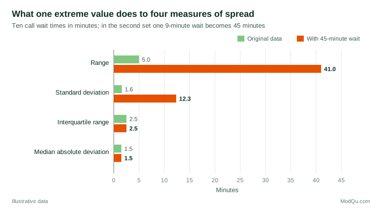
Figure 2 illustrates the effect with ten hypothetical call-centre wait times. When one 9-minute wait is replaced by a 45-minute wait, perhaps a system failure or a data-entry error, the range rises from 5 to 41 minutes and the standard deviation from 1.6 to 12.3 minutes. The interquartile range and the median absolute deviation do not change at all.
Robust alternatives
When data contain outliers or come from a skewed distribution, robust measures of spread give a more faithful picture of typical variation.
- The median absolute deviation (MAD) is the median of the absolute distances from the median. Multiplied by about 1.4826, it estimates the standard deviation for normally distributed data while resisting outliers. Its breakdown point is 50%, the highest possible, meaning almost half the data can be contaminated before it fails. Rousseeuw and Croux (1993) noted that the MAD is not very efficient for normal data and proposed alternative estimators that keep the high breakdown point with better efficiency.
- The mean absolute deviation averages the absolute distances from the mean rather than the squared ones. Gorard (2005), revisiting a debate that dates back to the early twentieth century, argued that it is easier to understand and less distorted by occasional errors in real data than the standard deviation.
- The interquartile range, described above, is robust to anything that happens in the outer quarters of the data.
These measures are also useful for screening. Leys et al. (2013) showed that the common rule of flagging observations more than two or three standard deviations from the mean is undermined by the very outliers it seeks, because they inflate the mean and the standard deviation. They recommended a criterion based on the median and the MAD instead, with 2.5 as a reasonable default threshold.
Practical guidance for survey and business data
- Always report spread alongside the centre. A mean without a standard deviation, IQR or distribution chart invites over-confident conclusions. Weissgerber et al. (2015) showed that bar charts of means can hide very different underlying distributions, and recommended showing the individual data points or the full distribution wherever possible.
- Choose the measure to suit the data. For roughly symmetric data without extreme values, the standard deviation is efficient and widely understood. For skewed measures such as spending or time on site, report the median with the IQR, or present both robust and classical figures.
- Add variances, not standard deviations, when combining independent sources of error, then take the square root at the end.
- Use survey weights. In a weighted sample, the mean and the variance should both be computed with the weights, or the spread will describe the sample rather than the population (Lohr, 2021).
- Watch for zero spread within respondents. In grid questions, a respondent who gives the same answer to every item has a within-person standard deviation of zero. Krosnick (1991) described this non-differentiation as a form of satisficing, and Kim et al. (2019) compared several indicators of straightlining, including measures based on the spread of a respondent's answers, for detecting low-quality responses.
- Estimate spread from summaries with care. When only a median and range are published, it is tempting to guess the standard deviation. Hozo et al. (2005) proposed simple estimation formulas, and Wan et al. (2014) showed that estimates which take account of sample size perform better. Label such estimates as approximations.
- Compute variance with a stable algorithm. The shortcut formula that subtracts the squared mean from the mean of squares can lose precision badly with large numbers. Chan et al. (1983) analysed the errors of the common algorithms, and the updating method of Welford (1962) remains a reliable one-pass approach for software that processes data in streams.
Common mistakes
- Comparing ranges from samples of different sizes. Larger samples tend to have larger ranges even when the population spread is identical.
- Confusing standard deviation with standard error. The first describes people, the second the precision of an estimate (Altman & Bland, 2005).
- Applying the 68–95–99.7 rule to skewed data. The rule is a property of the normal distribution; Chebyshev's bounds are the safe fallback.
- Mixing population and sample formulas. Software functions differ on whether they divide by n or n − 1.
- Treating high spread as bad by definition. A polarised rating may reveal two segments that deserve different strategies.
- Ignoring the scale's limits. On a bounded scale, a mean near the top forces the standard deviation to be small.
Key takeaways
The range shows the observed extremes but is fragile. The variance uses every observation but has squared units. The standard deviation returns spread to the original units and is the standard summary, provided the data are not heavily skewed or contaminated; for messy data, the IQR and MAD are valuable companions. Report spread with every average, keep standard deviations and standard errors distinct, and look at the distribution before trusting any single number.
References
Altman, D. G., & Bland, J. M. (2005). Standard deviations and standard errors. BMJ, 331(7521), 903. https://doi.org/10.1136/bmj.331.7521.903
Chan, T. F., Golub, G. H., & LeVeque, R. J. (1983). Algorithms for computing the sample variance: Analysis and recommendations. The American Statistician, 37(3), 242–247. https://doi.org/10.1080/00031305.1983.10483115
Cohen, J. (1988). Statistical power analysis for the behavioral sciences (2nd ed.). Routledge. https://doi.org/10.4324/9780203771587
Fisher, R. A. (1919). The correlation between relatives on the supposition of Mendelian inheritance. Transactions of the Royal Society of Edinburgh, 52(2), 399–433. https://doi.org/10.1017/S0080456800012163
Gorard, S. (2005). Revisiting a 90-year-old debate: The advantages of the mean deviation. British Journal of Educational Studies, 53(4), 417–430. https://doi.org/10.1111/j.1467-8527.2005.00304.x
Hampel, F. R. (1974). The influence curve and its role in robust estimation. Journal of the American Statistical Association, 69(346), 383–393. https://doi.org/10.1080/01621459.1974.10482962
Hozo, S. P., Djulbegovic, B., & Hozo, I. (2005). Estimating the mean and variance from the median, range, and the size of a sample. BMC Medical Research Methodology, 5(1), Article 13. https://doi.org/10.1186/1471-2288-5-13
Hyndman, R. J., & Fan, Y. (1996). Sample quantiles in statistical packages. The American Statistician, 50(4), 361–365. https://doi.org/10.1080/00031305.1996.10473566
Kim, Y., Dykema, J., Stevenson, J., Black, P., & Moberg, D. P. (2019). Straightlining: Overview of measurement, comparison of indicators, and effects in mail–web mixed-mode surveys. Social Science Computer Review, 37(2), 214–233. https://doi.org/10.1177/0894439317752406
Krosnick, J. A. (1991). Response strategies for coping with the cognitive demands of attitude measures in surveys. Applied Cognitive Psychology, 5(3), 213–236. https://doi.org/10.1002/acp.2350050305
Leys, C., Ley, C., Klein, O., Bernard, P., & Licata, L. (2013). Detecting outliers: Do not use standard deviation around the mean, use absolute deviation around the median. Journal of Experimental Social Psychology, 49(4), 764–766. https://doi.org/10.1016/j.jesp.2013.03.013
Lohr, S. L. (2021). Sampling: Design and analysis (3rd ed.). Chapman and Hall/CRC. https://doi.org/10.1201/9780429298899
Pearson, K. (1894). Contributions to the mathematical theory of evolution. Philosophical Transactions of the Royal Society of London. A, 185, 71–110. https://doi.org/10.1098/rsta.1894.0003
Rousseeuw, P. J., & Croux, C. (1993). Alternatives to the median absolute deviation. Journal of the American Statistical Association, 88(424), 1273–1283. https://doi.org/10.1080/01621459.1993.10476408
Saw, J. G., Yang, M. C. K., & Mo, T. C. (1984). Chebyshev inequality with estimated mean and variance. The American Statistician, 38(2), 130–132. https://doi.org/10.1080/00031305.1984.10483182
Stigler, S. M. (1986). The history of statistics: The measurement of uncertainty before 1900. Belknap Press of Harvard University Press.
Tippett, L. H. C. (1925). On the extreme individuals and the range of samples taken from a normal population. Biometrika, 17(3–4), 364–387. https://doi.org/10.1093/biomet/17.3-4.364
Tukey, J. W. (1977). Exploratory data analysis. Addison-Wesley.
Wan, X., Wang, W., Liu, J., & Tong, T. (2014). Estimating the sample mean and standard deviation from the sample size, median, range and/or interquartile range. BMC Medical Research Methodology, 14(1), Article 135. https://doi.org/10.1186/1471-2288-14-135
Wasserman, L. (2004). All of statistics: A concise course in statistical inference. Springer. https://doi.org/10.1007/978-0-387-21736-9
Weissgerber, T. L., Milic, N. M., Winham, S. J., & Garovic, V. D. (2015). Beyond bar and line graphs: Time for a new data presentation paradigm. PLOS Biology, 13(4), Article e1002128. https://doi.org/10.1371/journal.pbio.1002128
Welford, B. P. (1962). Note on a method for calculating corrected sums of squares and products. Technometrics, 4(3), 419–420. https://doi.org/10.1080/00401706.1962.10490022