
Statistics · Tests and models
Latent Class Analysis
How latent class analysis finds hidden groups in categorical survey answers, how to choose the number of classes, and how to profile, validate and report segments responsibly.
Survey analysts often suspect that a market is made up of a few distinct kinds of customers, even though no question asks people which kind they are. Some shoppers hunt for low prices, some research every purchase online, and some simply visit the same store every week. Latent class analysis (LCA) is a statistical model for exactly this situation. It assumes that respondents belong to a small number of unobserved groups, or latent classes, and it uses the pattern of answers to a set of categorical questions to estimate how large each group is and how its members tend to respond.
The idea goes back to Paul Lazarsfeld's work on latent structure analysis in the 1950s, summarised in the book by Lazarsfeld and Henry (1968). Practical estimation became possible when Goodman (1974) showed how to obtain maximum likelihood estimates and examined when the model is identified. Today LCA is a standard tool in sociology, health research, psychology and marketing, where it is widely used for segmentation (Collins & Lanza, 2009; Wedel & Kamakura, 2000). This article explains the model, works through an illustrative segmentation of shoppers, and sets out the decisions and mistakes that matter most in applied survey work.
What latent class analysis does
LCA starts from a set of observed categorical variables, called indicators. These are often yes/no items ("Do you use the store's loyalty app?") but can also have several unordered or ordered categories. The model assumes that a single categorical latent variable, class membership, explains the associations among these indicators. If you knew which class each person belonged to, the indicators would be unrelated to one another within each class. This assumption is called local independence or conditional independence, and it is the core of the model (Collins & Lanza, 2009).
The intuition is simple. LCA asks whether a small number of groups, each with its own typical pattern of answers, can reproduce these associations. If three groups are enough to account for how the items hang together, the analyst has a compact and interpretable description of the market.
LCA belongs to the wider family of finite mixture models, in which the population is treated as a mixture of subpopulations with different distributions (McLachlan & Peel, 2000). When the indicators are continuous rather than categorical, the same logic is usually called latent profile analysis.
The model
For a respondent with answers y = (y1, …, yJ) on J binary items and C classes, the probability of that answer pattern is
P(y) = Σc πc × Πj ρjcyj (1 − ρjc)1 − yj
Two kinds of parameter appear. The class proportions πc give the share of the population in each class, and they sum to 1. The item-response probabilities ρjc give the probability that a member of class c answers yes to item j. The product over items is where local independence enters: within a class, the probability of a whole answer pattern is just the product of the separate item probabilities. The sum over classes reflects that we do not know which class generated the pattern.
Parameters are estimated by maximum likelihood, usually with the expectation-maximisation (EM) algorithm (Dempster et al., 1977). EM alternates between estimating each respondent's probability of belonging to each class, given the current parameters, and updating the parameters, given those probabilities. Once the model is fitted, Bayes' theorem gives every respondent a posterior class membership probability:
P(class = c | y) = πc P(y | c) ÷ P(y)
These probabilities show not only which class a person most probably belongs to, but also how certain that assignment is.
The number of free parameters grows quickly. With J binary items and C classes there are (C − 1) class proportions plus C × J item probabilities. Six items and three classes give 2 + 18 = 20 parameters, while six classes give 41. A model is only identified if the data contain enough distinct answer patterns to pin these down; Goodman (1974) showed that some models with many classes relative to items cannot be estimated uniquely.
A worked example: shopper segments
Consider an illustrative survey of 1,200 grocery shoppers who answered six yes/no questions about their behaviour in the past month: whether they compared prices online, used a loyalty app, bought own-label products, shopped in store at least weekly, read product reviews, and paid more for an environmentally friendly product. The data are hypothetical, simulated for this article, and the models were fitted by maximum likelihood with 40 random starting values for each number of classes.
Choosing the number of classes
The analyst fits models with one to six classes and compares them. A one-class model is the baseline: it assumes all six items are independent across the whole sample, which is almost never true. Table 1 shows the log-likelihood, the number of parameters, two information criteria and the entropy statistic for each model.
| Classes | Log-likelihood | Parameters | AIC | BIC | Entropy |
|---|---|---|---|---|---|
| 1 | −4,793.0 | 6 | 9,598.0 | 9,628.5 | n/a |
| 2 | −4,532.4 | 13 | 9,090.7 | 9,156.9 | 0.74 |
| 3 | −4,404.1 | 20 | 8,848.2 | 8,950.0 | 0.69 |
| 4 | −4,400.0 | 27 | 8,854.0 | 8,991.5 | 0.76 |
| 5 | −4,396.9 | 34 | 8,861.8 | 9,034.9 | 0.75 |
| 6 | −4,393.8 | 41 | 8,869.6 | 9,078.3 | 0.74 |
The log-likelihood always improves when a class is added, because a more flexible model can always fit the sample a little better. Information criteria penalise that flexibility. The Akaike information criterion is AIC = −2 log L + 2k, and the Bayesian information criterion is BIC = −2 log L + k ln n, where k is the number of parameters and n the sample size (Akaike, 1974; Schwarz, 1978). BIC approximates a comparison of models by Bayes factors and penalises extra parameters more heavily than AIC in all but tiny samples (Kass & Raftery, 1995). A sample-size adjusted version of BIC, proposed by Sclove (1987), sits between the two.
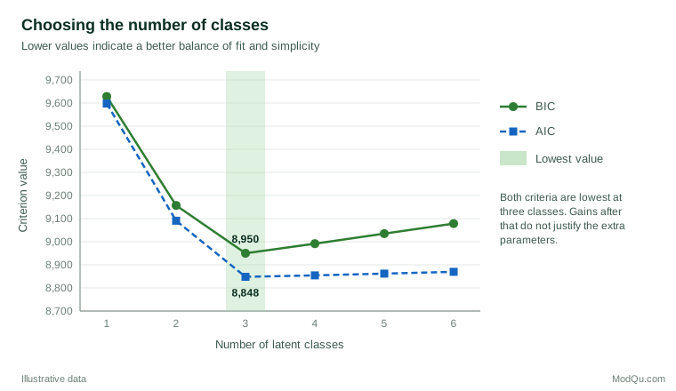
Here both criteria point to three classes (Figure 1). The improvement from three to four classes is only 4.1 log-likelihood points for seven extra parameters, which is not worth the added complexity. In real surveys the criteria often disagree, with AIC favouring more classes than BIC. In a large simulation study, Nylund et al. (2007) found that BIC was the best-performing information criterion for choosing the number of classes, that AIC tended to favour too many classes, and that the bootstrap likelihood ratio test (BLRT) was the most consistent indicator overall. The BLRT compares a model with C classes against one with C − 1 by simulating the distribution of the likelihood ratio, because the usual chi-square reference distribution does not apply when the simpler model sits on the boundary of the more complex one. The Lo-Mendell-Rubin test offers an analytic approximation for the same comparison (Lo et al., 2001).
Notice that entropy is higher for the four-class model than for the three-class model. Entropy summarises how clearly respondents are separated into classes, on a scale from 0 to 1. Entropy-based criteria for mixture models were examined by Celeux and Soromenho (1996), among others. Entropy describes classification quality, but it is not a test of how many classes exist. Nylund-Gibson and Choi (2018) advise against using it to choose the number of classes; a model with more, smaller classes can be better separated without being a better description of the population.
Interpreting the classes
Figure 2 shows the item-response probabilities for the three-class solution. Interpreting a latent class model means reading these profiles and giving each class a short, honest label.
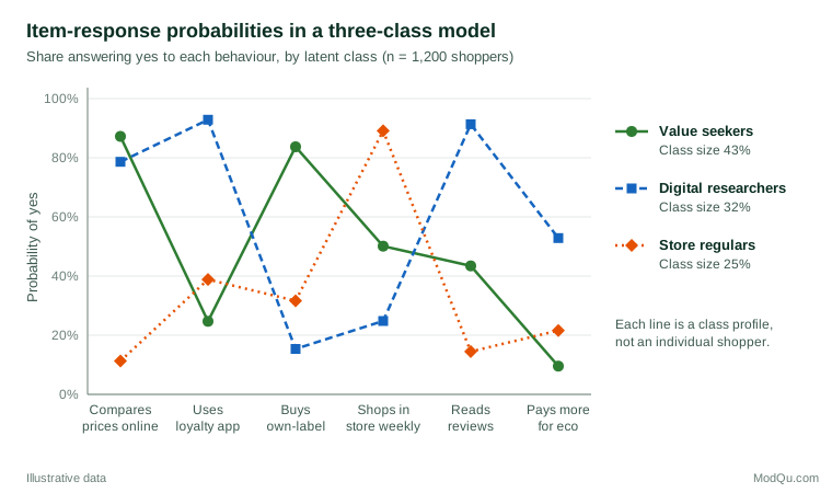
- Value seekers (43%) compare prices online (87%) and buy own-label products (84%), but rarely pay more for environmentally friendly options (10%).
- Digital researchers (32%) use the loyalty app (93%), read reviews (91%) and compare prices (79%). They are the class most willing to pay more for an environmentally friendly product (53%) and the least likely to buy own-label (15%).
- Store regulars (25%) are defined mainly by shopping in store every week (89%). They rarely compare prices online (11%) or read reviews (14%).
Collins and Lanza (2009) describe a well-defined class as one whose item-response probabilities are close to 0 or 1 (homogeneity) and clearly different from those of other classes (separation). In practice, analysts often treat values above about 0.7 or below about 0.3 as clearly high or low, and values in between as not distinguishing. Labels should follow the profile rather than the analyst's hopes. The value seekers' 50% chance of shopping in store weekly, for example, says nothing distinctive about them, so it should not feature in their name.
Classifying respondents
Each respondent receives three posterior probabilities. A shopper who compares prices online and buys own-label, but answers no to the other four questions, has a 99% posterior probability of being a value seeker. A shopper who compares prices, uses the app and reads reviews has a 96% probability of being a digital researcher. But a shopper who compares prices and shops in store weekly, and answers no to everything else, has a 62% probability of being a value seeker and a 37% probability of being a store regular. This person does not fit neatly into one class.
The average posterior probability for those assigned to each class (0.86, 0.89 and 0.85 here) is a useful summary of classification quality, and values above about 0.7 or 0.8 are commonly treated as adequate. The point to remember is that assignment is uncertain. Every time a respondent is placed in the most likely class, some are placed in the wrong one, and treating the assignments as known facts carries that error into later analysis.
Relating classes to other variables
Most business questions go beyond describing the classes. Analysts want to know whether digital researchers are younger, whether store regulars are more loyal, or whether value seekers spend less. The tempting approach is to export each respondent's most likely class and cross-tabulate it with age or spending. Bolck et al. (2004) showed that this "classify and analyse" approach systematically underestimates the relationships between class membership and other variables, because misclassification dilutes the differences between classes.
Two better routes are available. The first includes covariates such as age or region directly in the latent class model, so that class membership is predicted by a multinomial logistic regression estimated at the same time as the classes. This is statistically efficient, but adding covariates can change the classes themselves, which is undesirable if the segments are meant to be defined by behaviour alone. The second is a corrected three-step approach: fit the measurement model first, assign respondents using their posterior probabilities, then estimate the relationship with covariates or outcomes while correcting for known classification error (Vermunt, 2010). Asparouhov and Muthén (2014) describe how these corrections are implemented in widely used software, including versions for distal outcomes such as spending or satisfaction. For most applied segmentation, a corrected three-step method is the safer default.
Practical guidance for survey and business data
Choosing indicators
The classes can only be as good as the indicators that define them. Choose items that reflect the construct you want to segment on, such as shopping behaviour, attitudes or needs, and keep demographics out of the indicator set unless they are genuinely part of the definition. Items that almost everyone answers the same way contribute little, and redundant items that ask the same question twice are likely to violate local independence. Between about five and fifteen indicators is typical for survey segmentation, although more is possible with large samples.
Sample size and class separation
There is no single minimum sample size. The ability to detect the right number of classes depends on how distinct the classes are, how many indicators there are and how small the smallest class is. Simulation studies show that power to detect the correct number of classes depends strongly on separation: well-separated classes can be recovered with modest samples, while poorly separated ones may need far larger samples (Tein et al., 2013). Dziak et al. (2014) provide tables relating effect size, sample size and the power of the bootstrap likelihood ratio test. Very small classes, such as those holding less than about 5% of the sample, deserve suspicion: they may be real niches, but they may also be artefacts of a few unusual response patterns.
Estimation
The likelihood of a latent class model often has several local maxima, so a single run of the EM algorithm can stop at a poor solution (McLachlan & Peel, 2000). Always use many random starting values and check that the best log-likelihood is reached repeatedly. If the best value appears only once, the solution is not trustworthy and more starts, or a simpler model, are needed. Item-response probabilities that sit exactly at 0 or 1 are known as boundary estimates; a few are harmless, but many suggest the model has more classes than the data can support.
Missing data and survey design
LCA estimated by maximum likelihood can use respondents with some missing indicators, under the assumption that data are missing at random (Little & Rubin, 2019). This is usually better than dropping incomplete cases. When the data come from a weighted or complex sample, survey weights should be used in estimation so that class proportions describe the target population, and standard errors should reflect the design (Lumley, 2010). Unweighted class sizes from an unbalanced sample can be seriously misleading.
Checking local independence
Local independence is an assumption, not a given. Bivariate residuals, which compare observed and expected associations between each pair of indicators within the fitted model, show where it fails. Large residuals for a pair of items suggest either that a further class is needed or that the two items share something the classes do not explain, such as similar wording. Collins and Lanza (2009) and Hagenaars and McCutcheon (2002) describe ways to handle such dependence, including allowing a direct association between the two items.
Software
LCA is available in specialist packages such as Latent GOLD and Mplus, and in free software. The poLCA package for R, described by Linzer and Lewis (2011), fits latent class models to polytomous indicators and handles covariates, multiple starting values and missing data.
LCA compared with cluster analysis
Many segmentation projects use k-means or hierarchical cluster analysis. These methods group respondents by distance, without a probability model. LCA differs in four useful ways. It provides formal criteria for choosing the number of classes; it handles categorical indicators naturally rather than treating them as numbers; it gives each respondent a probability of membership rather than a hard label; and it does not depend on how variables are scaled. Wedel and Kamakura (2000) review the mixture approach to market segmentation and its advantages over heuristic clustering. The cost is stronger assumptions, especially local independence, and heavier computation. Neither approach discovers "true" segments automatically.
Common mistakes
- Choosing the number of classes by a single statistic. Information criteria, likelihood ratio tests, class sizes and interpretability should be weighed together (Nylund-Gibson & Choi, 2018). A solution that no one can describe is not useful, however good its BIC.
- Using entropy to pick the model. Entropy measures separation, not fit.
- Treating modal assignment as certain. Classify-and-analyse methods understate relationships with other variables (Bolck et al., 2004). Use corrected three-step or one-step methods.
- Reifying the classes. A latent class is a model-based summary of response patterns. Labels such as "value seekers" are convenient names, not discoveries of natural kinds, and different indicator sets would produce different classes.
- Relying on a single starting value. Local maxima are common and can produce misleading solutions.
- Ignoring weights and design. Class proportions from unweighted data describe the sample, not the market.
- Not validating. Check that the solution replicates in a holdout sample or in a later wave, and that the classes differ on outcomes they were not built from, such as spending or retention.
Reporting a latent class analysis
Good reporting lets a reader judge the solution. Weller et al. (2020) recommend describing the indicators and their coding, the software and estimation settings, including the number of random starts, and a table of fit statistics for all models compared. Report the item-response probabilities for the chosen model, class sizes, entropy or average posterior probabilities, and how classes were related to covariates or outcomes. For business readers, a profile chart like Figure 2 and a one-line description of each class usually communicate more than tables of parameters, but the technical material should remain available.
Key takeaways
Latent class analysis turns patterns of categorical survey answers into a small set of probabilistic segments. Its model is simple: a few unobserved groups, each with its own probabilities of answering yes, and answers independent within each group. Its strengths are formal model comparison, natural handling of categorical data, and honest measures of classification uncertainty. Use many starting values, compare models with BIC and likelihood ratio tests rather than entropy, weight the data where the design requires it, and relate classes to other variables with methods that correct for misclassification. Above all, treat the classes as a useful model of the market rather than as fixed groups waiting to be found.
References
Akaike, H. (1974). A new look at the statistical model identification. IEEE Transactions on Automatic Control, 19(6), 716–723. https://doi.org/10.1109/TAC.1974.1100705
Asparouhov, T., & Muthén, B. (2014). Auxiliary variables in mixture modeling: Three-step approaches using Mplus. Structural Equation Modeling: A Multidisciplinary Journal, 21(3), 329–341. https://doi.org/10.1080/10705511.2014.915181
Bolck, A., Croon, M., & Hagenaars, J. (2004). Estimating latent structure models with categorical variables: One-step versus three-step estimators. Political Analysis, 12(1), 3–27. https://doi.org/10.1093/pan/mph001
Celeux, G., & Soromenho, G. (1996). An entropy criterion for assessing the number of clusters in a mixture model. Journal of Classification, 13(2), 195–212. https://doi.org/10.1007/BF01246098
Collins, L. M., & Lanza, S. T. (2009). Latent class and latent transition analysis: With applications in the social, behavioral, and health sciences. Wiley. https://doi.org/10.1002/9780470567333
Dempster, A. P., Laird, N. M., & Rubin, D. B. (1977). Maximum likelihood from incomplete data via the EM algorithm. Journal of the Royal Statistical Society Series B: Statistical Methodology, 39(1), 1–22. https://doi.org/10.1111/j.2517-6161.1977.tb01600.x
Dziak, J. J., Lanza, S. T., & Tan, X. (2014). Effect size, statistical power, and sample size requirements for the bootstrap likelihood ratio test in latent class analysis. Structural Equation Modeling: A Multidisciplinary Journal, 21(4), 534–552. https://doi.org/10.1080/10705511.2014.919819
Goodman, L. A. (1974). Exploratory latent structure analysis using both identifiable and unidentifiable models. Biometrika, 61(2), 215–231. https://doi.org/10.1093/biomet/61.2.215
Hagenaars, J. A., & McCutcheon, A. L. (Eds.). (2002). Applied latent class analysis. Cambridge University Press. https://doi.org/10.1017/CBO9780511499531
Kass, R. E., & Raftery, A. E. (1995). Bayes factors. Journal of the American Statistical Association, 90(430), 773–795. https://doi.org/10.1080/01621459.1995.10476572
Lazarsfeld, P. F., & Henry, N. W. (1968). Latent structure analysis. Houghton Mifflin.
Linzer, D. A., & Lewis, J. B. (2011). poLCA: An R package for polytomous variable latent class analysis. Journal of Statistical Software, 42(10), 1–29. https://doi.org/10.18637/jss.v042.i10
Little, R. J. A., & Rubin, D. B. (2019). Statistical analysis with missing data (3rd ed.). Wiley. https://doi.org/10.1002/9781119482260
Lo, Y., Mendell, N. R., & Rubin, D. B. (2001). Testing the number of components in a normal mixture. Biometrika, 88(3), 767–778. https://doi.org/10.1093/biomet/88.3.767
Lumley, T. (2010). Complex surveys: A guide to analysis using R. Wiley. https://doi.org/10.1002/9780470580066
McLachlan, G., & Peel, D. (2000). Finite mixture models. Wiley. https://doi.org/10.1002/0471721182
Nylund, K. L., Asparouhov, T., & Muthén, B. O. (2007). Deciding on the number of classes in latent class analysis and growth mixture modeling: A Monte Carlo simulation study. Structural Equation Modeling: A Multidisciplinary Journal, 14(4), 535–569. https://doi.org/10.1080/10705510701575396
Nylund-Gibson, K., & Choi, A. Y. (2018). Ten frequently asked questions about latent class analysis. Translational Issues in Psychological Science, 4(4), 440–461. https://doi.org/10.1037/tps0000176
Schwarz, G. (1978). Estimating the dimension of a model. The Annals of Statistics, 6(2), 461–464. https://doi.org/10.1214/aos/1176344136
Sclove, S. L. (1987). Application of model-selection criteria to some problems in multivariate analysis. Psychometrika, 52(3), 333–343. https://doi.org/10.1007/BF02294360
Tein, J.-Y., Coxe, S., & Cham, H. (2013). Statistical power to detect the correct number of classes in latent profile analysis. Structural Equation Modeling: A Multidisciplinary Journal, 20(4), 640–657. https://doi.org/10.1080/10705511.2013.824781
Vermunt, J. K. (2010). Latent class modeling with covariates: Two improved three-step approaches. Political Analysis, 18(4), 450–469. https://doi.org/10.1093/pan/mpq025
Wedel, M., & Kamakura, W. A. (2000). Market segmentation: Conceptual and methodological foundations (2nd ed.). Springer. https://doi.org/10.1007/978-1-4615-4651-1
Weller, B. E., Bowen, N. K., & Faubert, S. J. (2020). Latent class analysis: A guide to best practice. Journal of Black Psychology, 46(4), 287–311. https://doi.org/10.1177/0095798420930932