
Statistics · Survey statistics
Inter-Rater Reliability: Cohen's Kappa and Related Measures
How to check whether two or more people code survey answers consistently, how Cohen's kappa corrects for chance agreement, why it can mislead, and which related measures to use instead.
Much of the value in survey data lies in answers that a person has to judge. Open-ended comments are sorted into themes, interviews are coded for mentions of competitors, and call recordings are rated for politeness. Whenever a human judgement turns raw material into a category or a score, a natural question follows: would a different, equally trained person have made the same judgement? Inter-rater reliability is the statistical answer to that question. It tells a research team whether its coding frame and its coders produce results that are reproducible, rather than results that depend on who happened to do the coding.
The best-known measure is Cohen's kappa (Cohen, 1960), which compares how often two raters agree with how often they would agree by chance alone. Kappa is widely used and widely misunderstood. This article explains how it works, shows where it misleads, and sets out the related measures that suit other designs: weighted kappa for ordered categories, Fleiss' kappa and Krippendorff's alpha for several coders, and the intraclass correlation for numeric ratings.
Why agreement matters in survey and business research
Reliability is a precondition for validity. If two coders cannot agree whether a comment is about price or about service, then the percentage of "price complaints" in a report partly reflects the coder rather than the customer. Disagreement also adds noise that weakens relationships with other variables, such as a link between service complaints and churn.
Reliability checks test the coding frame (low agreement on a category often means its definition is vague), calibrate coders before the main coding begins, and document quality for clients and reviewers. Lombard et al. (2002) reviewed published content analyses in mass communication research and found that many reported no reliability assessment at all, or reported it in ways that could not be checked.
Percentage agreement and its problem
The simplest measure is percentage agreement: the share of items on which two coders chose the same category. It is easy to compute and easy to explain, but it has a serious flaw. Some agreement happens by chance. If two coders each assign "yes" to 90% of items at random, without reading them, they will still agree on about 82% of items (0.9 × 0.9 + 0.1 × 0.1 = 0.82). A high percentage agreement can therefore hide coding that carries little real information, especially when one category dominates.
Chance-corrected measures address this by asking how much better than chance the coders did. The idea predates Cohen: Bennett et al. (1954) proposed a coefficient that assumes all categories are equally likely by chance, and Scott (1955) proposed his pi coefficient for content analysis, which estimates chance agreement from the pooled category distribution of both coders. Cohen's version, which estimates chance from each coder's own distribution, became the standard.
Cohen's kappa
Kappa compares observed agreement, po, with the agreement expected by chance, pe:
κ = (po − pe) ÷ (1 − pe)
The numerator is the agreement achieved beyond chance; the denominator is the most agreement beyond chance that was possible. A kappa of 1 means perfect agreement. A kappa of 0 means agreement no better than chance, and negative values mean systematic disagreement. Expected agreement is computed from the marginal totals, the share of items each coder put in each category:
pe = Σk pA,k × pB,k
where pA,k and pB,k are the proportions of items that coders A and B assigned to category k. This is the agreement two coders would reach if they kept their own category frequencies but assigned items independently of content.
A worked example
Suppose, hypothetically, that a retailer's customer survey collects 200 open-ended answers to the question "What is the main reason for your rating?". Two trained coders independently assign each answer to one of four themes: price, service, product or other. Figure 1 shows the resulting agreement matrix.
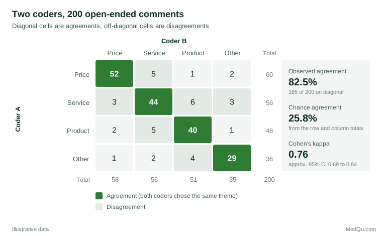
The coders agree on 52 + 44 + 40 + 29 = 165 comments, so po = 165 ÷ 200 = 0.825. Chance agreement uses the totals. For price, coder A used the category for 60 of 200 comments (30%) and coder B for 58 (29%), so chance agreement on price is 0.30 × 0.29 = 0.087. Repeating this for service (0.28 × 0.28 = 0.078), product (0.24 × 0.255 = 0.061) and other (0.18 × 0.175 = 0.032) and adding gives pe = 0.258. Then:
κ = (0.825 − 0.258) ÷ (1 − 0.258) = 0.567 ÷ 0.742 ≈ 0.76
The coders closed about three-quarters of the gap between chance and perfect agreement. A rough standard error, following Cohen (1960), is √[po(1 − po) ÷ (n(1 − pe)²)] ≈ 0.036, which gives an approximate 95% confidence interval of 0.69 to 0.84. With only 200 items, kappa is estimated with useful but not high precision.
The matrix is as informative as the summary. Most disagreements involve service and product: six comments that coder A called service were called product by coder B, and five went the other way. That pattern suggests the coding frame needs a clearer rule for comments such as "the staff could not tell me how the product worked", which mention both. Category-level checks, such as computing kappa for each theme against all the others, help to locate such problems.
Interpreting kappa: benchmarks and their limits
Kappa values are usually compared with verbal benchmarks. The most cited are those of Landis and Koch (1977): below 0 poor, 0 to 0.20 slight, 0.21 to 0.40 fair, 0.41 to 0.60 moderate, 0.61 to 0.80 substantial and 0.81 to 1 almost perfect. Fleiss et al. (2003) offered a coarser scheme in which values above 0.75 are excellent, 0.40 to 0.75 fair to good, and below 0.40 poor. By either scheme, the example's 0.76 is good.
These labels were proposed as rough conventions, not as tested standards, and they disagree with each other. McHugh (2012) argues that the Landis and Koch bands are too lenient for health research, where a kappa of 0.41 would mean that a large share of the coded data is unreliable, and suggests treating values below 0.60 as inadequate. In content analysis, Krippendorff (2004) recommends relying only on variables with reliability of at least 0.80, and drawing only tentative conclusions between 0.667 and 0.80. Lombard et al. (2002) suggest that 0.80 is acceptable in most situations and lower values only for exploratory work.
A sensible rule for business research is to set the threshold before coding begins, according to the use of the data: a variable that drives a headline figure deserves a higher standard than one used to explore themes. Report the confidence interval and check its lower limit against the threshold.
When kappa misleads: prevalence and bias
Kappa depends not only on how well coders agree but also on how the categories are distributed. Feinstein and Cicchetti (1990) described two paradoxes that follow from this. The first is the most important in practice: high agreement can coexist with low kappa when one category is much more common than the other.
Consider a hypothetical check of 500 customer comments, in which two coders flag whether each comment mentions a named competitor. They both flag the same 10 comments, each flags 15 others that the other does not, and they agree on 460 comments with no mention. Observed agreement is 470 ÷ 500 = 94%. But because each coder flags only 5% of comments, chance agreement is 0.05 × 0.05 + 0.95 × 0.95 = 0.905, and kappa is (0.94 − 0.905) ÷ (1 − 0.905) ≈ 0.37, which is merely "fair". If the same 94% agreement had occurred with a 50:50 split, chance agreement would be 0.50 and kappa would be 0.88. Figure 2 shows this relationship for three levels of observed agreement.
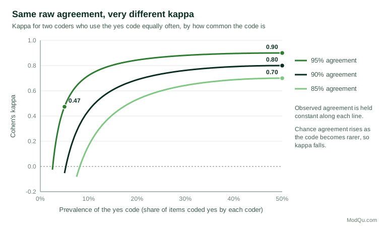
This is not an error in the formula. When a code is rare, most agreement is on the easy "no" side; what matters is agreement on the few "yes" cases. In the competitor example they agree on only 10 of the 40 comments that either of them flagged, which is genuinely weak. Kappa is therefore telling a useful truth, but it is a truth about the rare category, and it cannot be compared fairly with a kappa from a balanced category.
The second paradox concerns bias, meaning that the coders use categories at different rates. Holding agreement constant, kappa is higher when the coders' marginal distributions differ than when they match, which seems backwards. Byrt et al. (1993) proposed reporting a prevalence index and a bias index alongside kappa, together with a prevalence-adjusted bias-adjusted kappa (PABAK), which for two categories equals 2po − 1. In the competitor example, PABAK is 2 × 0.94 − 1 = 0.88. Cicchetti and Feinstein (1990) recommended a different remedy: report the separate agreement on positive and on negative cases. Here, positive agreement is 2 × 10 ÷ (2 × 10 + 15 + 15) = 0.40, while negative agreement is 0.97. These two figures make the real problem obvious.
Sim and Wright (2005) give a clear review of these issues. Their advice, and the advice of most later authors, is not to abandon kappa, but to report it with the agreement table, the prevalence of each category and, where the distribution is skewed, positive and negative agreement.
Weighted kappa for ordered categories
Ordinary kappa treats every disagreement as equally serious. For ordered categories, such as sentiment coded as negative, neutral or positive, or a quality rating from 1 to 5, that is too harsh: confusing "negative" with "neutral" is a smaller error than confusing "negative" with "positive". Weighted kappa (Cohen, 1968) gives partial credit to near misses by assigning a weight to each cell of the agreement table.
Two weighting schemes are common. Linear weights penalise a disagreement in proportion to the number of categories between the two codes; quadratic weights penalise it in proportion to the square of that distance, so adjacent disagreements cost little and distant ones a great deal. Fleiss and Cohen (1973) showed that, under certain conditions, quadratically weighted kappa is equivalent to the intraclass correlation coefficient, which links it to the reliability measures used for numeric ratings.
As a hypothetical example, suppose two coders rate the sentiment of 150 comments on a three-point scale and agree on 78% of them, with most disagreements between adjacent categories. Unweighted kappa is 0.66, linearly weighted kappa is 0.70 and quadratically weighted kappa is 0.75. The choice of weights should be made, and stated, before the results are seen, because a team that tries all three and reports the highest is overstating its reliability. Weighted kappa should not be used for nominal categories such as themes, where there is no meaningful distance between price and service.
More than two raters
Many coding projects use more than two coders, often with each item coded by a different subset, so Cohen's kappa does not apply directly.
Fleiss' kappa (Fleiss, 1971) extends Scott's pi to any fixed number of raters per item. It compares the average agreement among pairs of raters on each item with the agreement expected from the overall category distribution. It does not require the same raters to code every item, but it does require the same number of ratings per item.
Krippendorff's alpha is more general still. It handles any number of coders, missing ratings, and nominal, ordinal, interval or ratio data within one framework, and it reduces to a close relative of Scott's pi in the simplest case. Hayes and Krippendorff (2007) argued that alpha should become the standard reliability measure for coded data, precisely because one coefficient can serve so many designs. For teams coding thousands of open-ended answers with rotating staff, alpha is often the most practical choice.
Hallgren (2012) gives a readable tutorial on choosing among these measures.
Numeric ratings: the intraclass correlation
When raters give numeric scores, such as an interviewer's rating of respondent engagement on a 0 to 10 scale or a panel's scoring of advertising concepts, kappa is not the right tool. The intraclass correlation coefficient (ICC) estimates the share of variation in ratings that reflects true differences between the items rated, rather than differences between raters or random error.
Shrout and Fleiss (1979) set out several forms of the ICC, which differ in whether raters are treated as a random sample or as the only raters of interest, whether systematic differences between raters count against reliability (absolute agreement) or not (consistency), and whether the reliability of single ratings or of averaged ratings is wanted. These forms can give quite different values from the same data, so the form must be reported. Koo and Li (2016) provide a practical guide to choosing among them and suggest that values below 0.5 indicate poor reliability, 0.5 to 0.75 moderate, 0.75 to 0.9 good, and above 0.9 excellent.
A plain correlation is not a substitute: two raters can correlate perfectly while one always scores two points higher. For questions about whether two raters or methods give interchangeable numbers, Bland and Altman (1986) proposed plotting the differences between paired measurements against their averages and reporting limits of agreement, an approach now standard in measurement studies.
Alternatives to Cohen's kappa for skewed categories
Because of the prevalence problem, several alternative coefficients have been proposed. Brennan and Prediger (1981) discussed a "free-marginal" kappa, equivalent to the earlier coefficient of Bennett et al. (1954), which assumes chance agreement of 1 ÷ k for k categories. It suits designs in which coders are not constrained to use categories at any particular rate. Gwet (2008) proposed the AC1 statistic, which defines chance agreement in a way that stays low when one category dominates, so it behaves more stably than kappa under high prevalence. Critics respond that these coefficients make reliability look better precisely where coders struggle with the rare category, and Krippendorff (2004) warns against measures that ignore the coders' actual distributions. No single coefficient answers every question, so a good report gives the raw table so that readers can compute others.
Designing a reliability check
The coefficient matters less than the design of the check that produces it. Kottner et al. (2011) set out the Guidelines for Reporting Reliability and Agreement Studies (GRRAS), which ask researchers to describe the items, the raters, the sampling of both, the rating process and the statistical methods. Translated into practical steps for coding survey data:
- Code independently. Coders must not discuss items or see each other's codes during the reliability sample. Agreement reached by consensus is not inter-rater reliability.
- Use a representative sample of items. Draw the reliability sample at random from the full set, and make it large enough to include the rarer categories. With a category that occurs in 5% of items, a sample of 100 contains only about five examples, which is too few to judge agreement on that category. Sim and Wright (2005) discuss sample size calculations for kappa.
- Test the coding frame first. Run a pilot round, review the disagreements, refine the definitions, then measure reliability on fresh items.
- Monitor drift. In long projects, repeat the check on a fresh sample at intervals.
- Report fully. Give the coefficient, its confidence interval, the number of items and coders, the category distribution and the agreement table or the category-level results.
O'Connor and Joffe (2020) review the debate over whether intercoder reliability belongs in qualitative analysis and conclude that it can be useful, particularly in team-based coding of large data sets, as long as it supports rather than replaces reflection on the meaning of the codes.
Common mistakes
- Reporting percentage agreement alone. It overstates reliability whenever one category is common, as the competitor example shows.
- Quoting a single benchmark label. Calling 0.62 "substantial" says little without the confidence interval, the prevalence and the purpose of the data.
- Comparing kappas across categories or studies with different prevalence. A kappa of 0.5 for a rare code and 0.8 for a common one may reflect similar coder skill.
- Using Cohen's kappa when raters differ across items, instead of Fleiss' kappa or Krippendorff's alpha.
- Measuring reliability on consensus-coded items, or on the training items used to refine the frame.
Key takeaways
Inter-rater reliability tells a research team whether coded survey data reflect the respondents or the coders. Cohen's kappa removes the agreement expected by chance and remains the standard measure for two coders and nominal categories. It must be read with care: kappa falls sharply when a category is rare, its benchmark labels are conventions, and its precision depends on the number of items checked. Weighted kappa suits ordered categories, Fleiss' kappa and Krippendorff's alpha suit several coders, and the intraclass correlation suits numeric ratings. Above all, a sound reliability check needs independent coding of a representative sample, a threshold set in advance, and a full report that includes the agreement table.
References
Bennett, E. M., Alpert, R., & Goldstein, A. C. (1954). Communications through limited-response questioning. Public Opinion Quarterly, 18(3), 303–308. https://doi.org/10.1086/266520
Bland, J. M., & Altman, D. G. (1986). Statistical methods for assessing agreement between two methods of clinical measurement. The Lancet, 327(8476), 307–310. https://doi.org/10.1016/S0140-6736(86)90837-8
Brennan, R. L., & Prediger, D. J. (1981). Coefficient kappa: Some uses, misuses, and alternatives. Educational and Psychological Measurement, 41(3), 687–699. https://doi.org/10.1177/001316448104100307
Byrt, T., Bishop, J., & Carlin, J. B. (1993). Bias, prevalence and kappa. Journal of Clinical Epidemiology, 46(5), 423–429. https://doi.org/10.1016/0895-4356(93)90018-V
Cicchetti, D. V., & Feinstein, A. R. (1990). High agreement but low kappa: II. Resolving the paradoxes. Journal of Clinical Epidemiology, 43(6), 551–558. https://doi.org/10.1016/0895-4356(90)90159-M
Cohen, J. (1960). A coefficient of agreement for nominal scales. Educational and Psychological Measurement, 20(1), 37–46. https://doi.org/10.1177/001316446002000104
Cohen, J. (1968). Weighted kappa: Nominal scale agreement provision for scaled disagreement or partial credit. Psychological Bulletin, 70(4), 213–220. https://doi.org/10.1037/h0026256
Feinstein, A. R., & Cicchetti, D. V. (1990). High agreement but low kappa: I. The problems of two paradoxes. Journal of Clinical Epidemiology, 43(6), 543–549. https://doi.org/10.1016/0895-4356(90)90158-L
Fleiss, J. L. (1971). Measuring nominal scale agreement among many raters. Psychological Bulletin, 76(5), 378–382. https://doi.org/10.1037/h0031619
Fleiss, J. L., & Cohen, J. (1973). The equivalence of weighted kappa and the intraclass correlation coefficient as measures of reliability. Educational and Psychological Measurement, 33(3), 613–619. https://doi.org/10.1177/001316447303300309
Fleiss, J. L., Levin, B., & Paik, M. C. (2003). Statistical methods for rates and proportions (3rd ed.). Wiley. https://doi.org/10.1002/0471445428
Gwet, K. L. (2008). Computing inter-rater reliability and its variance in the presence of high agreement. British Journal of Mathematical and Statistical Psychology, 61(1), 29–48. https://doi.org/10.1348/000711006X126600
Hallgren, K. A. (2012). Computing inter-rater reliability for observational data: An overview and tutorial. Tutorials in Quantitative Methods for Psychology, 8(1), 23–34. https://doi.org/10.20982/tqmp.08.1.p023
Hayes, A. F., & Krippendorff, K. (2007). Answering the call for a standard reliability measure for coding data. Communication Methods and Measures, 1(1), 77–89. https://doi.org/10.1080/19312450709336664
Koo, T. K., & Li, M. Y. (2016). A guideline of selecting and reporting intraclass correlation coefficients for reliability research. Journal of Chiropractic Medicine, 15(2), 155–163. https://doi.org/10.1016/j.jcm.2016.02.012
Kottner, J., Audigé, L., Brorson, S., Donner, A., Gajewski, B. J., Hróbjartsson, A., Roberts, C., Shoukri, M., & Streiner, D. L. (2011). Guidelines for Reporting Reliability and Agreement Studies (GRRAS) were proposed. Journal of Clinical Epidemiology, 64(1), 96–106. https://doi.org/10.1016/j.jclinepi.2010.03.002
Krippendorff, K. (2004). Reliability in content analysis: Some common misconceptions and recommendations. Human Communication Research, 30(3), 411–433. https://doi.org/10.1111/j.1468-2958.2004.tb00738.x
Landis, J. R., & Koch, G. G. (1977). The measurement of observer agreement for categorical data. Biometrics, 33(1), 159–174. https://doi.org/10.2307/2529310
Lombard, M., Snyder-Duch, J., & Bracken, C. C. (2002). Content analysis in mass communication: Assessment and reporting of intercoder reliability. Human Communication Research, 28(4), 587–604. https://doi.org/10.1111/j.1468-2958.2002.tb00826.x
McHugh, M. L. (2012). Interrater reliability: The kappa statistic. Biochemia Medica, 22(3), 276–282. https://doi.org/10.11613/BM.2012.031
O'Connor, C., & Joffe, H. (2020). Intercoder reliability in qualitative research: Debates and practical guidelines. International Journal of Qualitative Methods, 19, Article 1609406919899220. https://doi.org/10.1177/1609406919899220
Scott, W. A. (1955). Reliability of content analysis: The case of nominal scale coding. Public Opinion Quarterly, 19(3), 321–325. https://doi.org/10.1086/266577
Shrout, P. E., & Fleiss, J. L. (1979). Intraclass correlations: Uses in assessing rater reliability. Psychological Bulletin, 86(2), 420–428. https://doi.org/10.1037/0033-2909.86.2.420
Sim, J., & Wright, C. C. (2005). The kappa statistic in reliability studies: Use, interpretation, and sample size requirements. Physical Therapy, 85(3), 257–268. https://doi.org/10.1093/ptj/85.3.257