
Statistics · Inference
Hypothesis Testing: Null, Alternative and Decision Rules
How a statistical test turns a business question into a null and an alternative hypothesis, a decision rule and two kinds of error, with a worked survey example and practical guidance.
Did the new packaging raise purchase intention, or is the difference between two survey cells just sampling noise? Hypothesis testing is the formal procedure statistics offers for questions of this kind. It sets up two competing statements about a population, fixes in advance a rule for choosing between them, and controls how often that rule leads to the wrong conclusion. The approach combines Fisher's (1925) significance tests with the decision framework of Neyman and Pearson (1933), and although the two schools disagreed on its interpretation, the combined procedure is what most textbooks and software now teach (Lehmann, 1993).
The null and the alternative hypothesis
Every test starts with two hypotheses about a population parameter, such as a mean, a proportion or a difference between groups.
- The null hypothesis (H0) is the default or "no effect" position: the new packaging and the old packaging produce the same purchase intention, the two regions have the same satisfaction score, the campaign did not change awareness.
- The alternative hypothesis (H1 or Ha) is what the analyst would conclude if the data contradict the null: the two versions differ.
The hypotheses are statements about the population, never about the sample. The question is whether a sample difference is large enough, given the sample size, to infer a real population difference.
An alternative can be two-sided (the versions differ in either direction) or one-sided (the new version is better). A one-sided test has more power to detect an effect in the stated direction, but it must be chosen before the data are seen and only when an effect in the other direction would genuinely lead to the same decision as no effect. In most market research, two-sided tests are the safer default.
Test statistics and decision rules
A test summarises the evidence in a single test statistic, usually the observed difference divided by its standard error. If the null hypothesis were true, the statistic would follow a known sampling distribution, such as the standard normal for a large-sample z-test or the t distribution for a t-test (Casella & Berger, 2002).
The decision rule says which values of the statistic lead to rejecting H0. It is fixed by choosing a significance level, α, which is the probability of rejecting the null when it is in fact true. With α = 0.05 and a two-sided z-test, the critical values are ±1.96:
Reject H0 if |z| ≥ 1.96; otherwise do not reject H0
An equivalent form of the rule compares the p-value with α: reject when p ≤ α. The level 0.05 is a convention, not a law; Fisher (1925) suggested it as a convenient benchmark, and a stricter or looser level can be justified by the costs of each kind of mistake.
Two kinds of error
Because the decision is made from a sample, it can be wrong in two ways (Neyman & Pearson, 1933).
| H0 true (no real effect) | H0 false (real effect) | |
|---|---|---|
| Reject H0 | Type I error (probability α) | Correct decision (power, 1 − β) |
| Do not reject H0 | Correct decision | Type II error (probability β) |
A Type I error is a false alarm: declaring a difference that does not exist. A Type II error is a missed effect. The statistical power of a test, 1 − β, is the probability of detecting an effect of a given size. Power rises with sample size, with the size of the true effect and with α. Cohen (1992) proposed 80% as a reasonable minimum.
A worked example
A hypothetical consumer panel study randomly shows 1,000 respondents the current pack and 1,000 a redesigned pack. Purchase intention ("definitely or probably would buy") is 40.0% for the current pack and 44.5% for the new one.
- Hypotheses. H0: the population proportions are equal. H1: they differ (two-sided).
- Decision rule. α = 0.05, so reject H0 if |z| ≥ 1.96.
- Test statistic. The pooled proportion is 42.25%, giving a standard error for the difference of 2.21 points:
z = (0.445 − 0.400) ÷ 0.0221 = 2.04
- Decision. Because 2.04 exceeds 1.96 (equivalently, p = 0.042), the null hypothesis is rejected. The 95% confidence interval for the lift runs from about 0.2 to 8.8 points.
The result is statistically significant, but the interval shows that the true lift could be almost nothing or quite large.
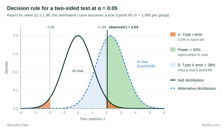
Figure 1 also shows why planning matters. If the true lift were exactly 5 points, this design would detect it only about 62% of the time. Roughly 1,530 respondents per group would be needed for 80% power, and about 4,230 per group to detect a 3-point lift with the same power.
Practical guidance for survey and business data
- Write the hypotheses and the rule before collecting data. State the outcome, the comparison, α and whether the test is one- or two-sided. Deciding these after seeing the results inflates the false-positive rate (Simmons et al., 2011).
- Plan the sample size from the smallest effect worth acting on. A power calculation turns a business threshold, such as "a 3-point lift pays for the redesign", into a required sample (Cohen, 1992).
- Report effect sizes and confidence intervals, not only "significant" or "not significant". The interval tells decision-makers how large the effect plausibly is.
- Adjust for many comparisons. Testing 20 brand attributes or 15 regions at α = 0.05 will produce false alarms by chance. Procedures that control the false discovery rate keep this in check (Benjamini & Hochberg, 1995).
- Use design-aware standard errors for weighted or clustered survey samples; simple formulas usually understate the uncertainty.
- Do not stop early on a good result. In online experiments, repeatedly checking and stopping as soon as p dips below 0.05 greatly inflates Type I error unless a sequential design is used (Kohavi et al., 2020).
Common mistakes
- Treating "not significant" as "no difference". Failing to reject H0 often reflects low power. Absence of evidence is not evidence of absence (Altman & Bland, 1995). To show that two versions are practically the same, use an equivalence test (Lakens, 2017).
- Confusing statistical and practical significance. With very large samples, trivial differences become significant. Cohen (1994) warned that the ritual of rejecting a null of exactly zero says little about whether an effect matters.
- Reading α as the chance the conclusion is wrong. α is the error rate when the null is true, not the probability that a particular significant result is a false alarm.
- Choosing a one-sided test after seeing the direction of the result. This quietly doubles the effective α.
Key takeaways
A hypothesis test pits a null hypothesis of no effect against an alternative, and uses a decision rule fixed in advance to choose between them. The significance level controls false alarms; power, driven mainly by sample size, controls missed effects. Used well, with pre-specified hypotheses, adequate samples, effect sizes, confidence intervals and corrections for multiple testing, the procedure gives business decisions a disciplined check against sampling noise (Lehmann & Romano, 2005).
References
Altman, D. G., & Bland, J. M. (1995). Absence of evidence is not evidence of absence. BMJ, 311(7003), 485. https://doi.org/10.1136/bmj.311.7003.485
Benjamini, Y., & Hochberg, Y. (1995). Controlling the false discovery rate: A practical and powerful approach to multiple testing. Journal of the Royal Statistical Society Series B: Statistical Methodology, 57(1), 289–300. https://doi.org/10.1111/j.2517-6161.1995.tb02031.x
Casella, G., & Berger, R. L. (2002). Statistical inference (2nd ed.). Duxbury.
Cohen, J. (1992). A power primer. Psychological Bulletin, 112(1), 155–159. https://doi.org/10.1037/0033-2909.112.1.155
Cohen, J. (1994). The earth is round (p < .05). American Psychologist, 49(12), 997–1003. https://doi.org/10.1037/0003-066X.49.12.997
Fisher, R. A. (1925). Statistical methods for research workers. Oliver and Boyd.
Kohavi, R., Tang, D., & Xu, Y. (2020). Trustworthy online controlled experiments: A practical guide to A/B testing. Cambridge University Press. https://doi.org/10.1017/9781108653985
Lakens, D. (2017). Equivalence tests: A practical primer for t tests, correlations, and meta-analyses. Social Psychological and Personality Science, 8(4), 355–362. https://doi.org/10.1177/1948550617697177
Lehmann, E. L. (1993). The Fisher, Neyman-Pearson theories of testing hypotheses: One theory or two? Journal of the American Statistical Association, 88(424), 1242–1249. https://doi.org/10.1080/01621459.1993.10476404
Lehmann, E. L., & Romano, J. P. (2005). Testing statistical hypotheses (3rd ed.). Springer. https://doi.org/10.1007/0-387-27605-X
Neyman, J., & Pearson, E. S. (1933). On the problem of the most efficient tests of statistical hypotheses. Philosophical Transactions of the Royal Society of London. Series A, 231(694–706), 289–337. https://doi.org/10.1098/rsta.1933.0009
Simmons, J. P., Nelson, L. D., & Simonsohn, U. (2011). False-positive psychology: Undisclosed flexibility in data collection and analysis allows presenting anything as significant. Psychological Science, 22(11), 1359–1366. https://doi.org/10.1177/0956797611417632