
Statistics · Inference
The Margin of Error in Survey Results
How the "plus or minus" figure on a survey is calculated, what drives it, what it leaves out, and how to report and plan for it in market research and business surveys.
"Forty-two percent of customers would pay more for faster delivery, with a margin of error of plus or minus 3 percentage points." Sentences like this appear in almost every published poll and many business survey reports. The margin of error is the most familiar single measure of survey precision, and it is useful. It is also narrower in meaning than most readers assume. This article explains how the margin of error is calculated, what makes it larger or smaller, which comparisons it does not cover, and why the real uncertainty in a survey is usually greater than the headline figure suggests.
What the margin of error is
The margin of error is the half-width of a confidence interval, usually a 95% interval, for an estimate from a sample. If a survey reports 42% ± 3 points, the 95% confidence interval runs from 39% to 45%. The underlying logic comes from probability sampling: when respondents are selected at random from a defined population, the variation of the estimate from sample to sample can be calculated from probability theory (Neyman, 1934; Kish, 1965).
For a proportion p estimated from a simple random sample of n people, the margin of error at the 95% level is:
MOE = 1.96 × √(p(1 − p) ÷ n)
The value 1.96 is the critical value from the normal distribution for 95% confidence; a 90% margin would use 1.645 and a 99% margin 2.576. The term under the square root is the variance of a single yes/no answer, p(1 − p), divided by the sample size. That variance is largest when p = 50%, so reports usually quote the maximum margin of error, calculated at 50%, as one figure for the whole survey (Lohr, 2021). A simple approximation follows: the maximum 95% margin is close to 1 ÷ √n. For 1,000 respondents, that is about 3.2 points; the exact figure is 3.1.
A worked example
Suppose a hypothetical retailer surveys a simple random sample of 1,000 customers from its loyalty database, and 420 say they would pay more for next-day delivery. The estimate is 42.0%, and its margin of error is:
MOE = 1.96 × √(0.42 × 0.58 ÷ 1,000) ≈ 1.96 × 0.0156 ≈ 3.1 points
So the 95% confidence interval runs from about 38.9% to 45.1%. The maximum margin, at 50%, would also round to 3.1 points. For smaller or larger proportions the margin shrinks: a 10% result from the same survey has a margin of only about 1.9 points. A survey report that quotes "± 3.1 points" for every question is therefore conservative for results far from 50%.
How sample size drives the margin
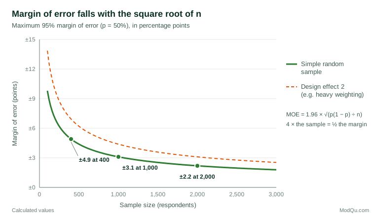
Because the sample size sits under a square root, precision improves with diminishing returns. Doubling the sample does not halve the margin; it takes four times the sample to do that. Figure 1 shows the curve, and the table below gives the maximum 95% margin for common sample sizes.
| Sample size | Maximum 95% margin of error |
|---|---|
| 100 | ± 9.8 points |
| 400 | ± 4.9 points |
| 600 | ± 4.0 points |
| 1,000 | ± 3.1 points |
| 1,500 | ± 2.5 points |
| 2,500 | ± 2.0 points |
| 10,000 | ± 1.0 point |
The practical consequence is that moving from 1,000 to 2,000 interviews roughly doubles the fieldwork cost but reduces the margin only from 3.1 to 2.2 points. Whether the extra precision is worth paying for depends on the decision the survey supports. A few hundred interviews can show whether a figure is nearer 30% or 60%; detecting a two-point change in market share takes several thousand.
Population size barely matters
A frequent surprise is that the size of the population hardly affects the margin of error. A random sample of 1,000 has much the same precision whether it is drawn from a city of 500,000 or a country of 40 million.
The exception is when the sample is a large fraction of a small population, as in many business-to-business and employee surveys. The margin is then multiplied by the finite population correction, √((N − n) ÷ (N − 1)), where N is the population size (Cochran, 1977). For a survey of 500 clients out of a total client base of 2,000, the correction is about 0.87, and the maximum margin falls from 4.4 to 3.8 points. When the sample is less than about 5% of the population, the correction makes little difference and is usually ignored.
Design effects, weighting and effective sample size
The formula above assumes a simple random sample with no weighting. Real surveys rarely meet that assumption. Clustered samples, in which respondents are selected in groups such as households, schools or stores, tend to contain people who resemble one another, which adds variance. Stratified samples can reduce variance. Weighting to correct for unequal selection probabilities or nonresponse almost always increases it (Kish, 1965; Lohr, 2021).
Kish (1965) summarised these effects with the design effect: the ratio of the actual variance of an estimate to the variance it would have under simple random sampling of the same size. The effective sample size is the actual sample size divided by the design effect. A survey of 1,000 with a design effect of 1.5 has the precision of a simple random sample of about 667, and a maximum margin of about 3.8 points rather than 3.1:
MOEdesign = MOESRS × √deff
For weighting alone, Kish (1992) gave a widely used approximation: the design effect due to weighting is about 1 + CV², where CV is the coefficient of variation of the weights. Weights with a CV of 0.7, which is common after weighting a panel sample to several population targets, imply a design effect of about 1.5. More exact standard errors come from Taylor linearisation or replication methods such as the jackknife (Wolter, 2007).
Many published margins of error ignore the design effect and quote the simple random sample figure. That understates the uncertainty. A good report states whether the margin has been adjusted and, if so, by how much (Valliant et al., 2018).
What "plus or minus 3 points" does not cover
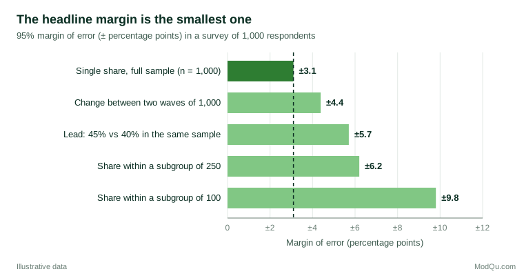
The headline margin applies to a single proportion estimated from the full sample. Many of the comparisons that readers actually care about have larger margins. Figure 2 compares several for a hypothetical survey of 1,000 respondents.
Subgroups
A subgroup estimate is based on only the respondents in that subgroup. If 250 of the 1,000 respondents are aged under 35, a result for that group has a maximum margin of about 6.2 points, twice the headline figure. A subgroup of 100 has a margin of about 9.8 points. Commentary on segments without subgroup margins invites over-interpretation.
The lead between two options
When a poll reports that option A has 45% and option B has 40%, readers often ask whether the 5-point lead exceeds the margin of error. The margin for the lead is not the headline margin, and it is not simply double it. Because the two shares come from the same respondents and are negatively correlated (a respondent who chooses A cannot also choose B), the variance of the difference is [pA + pB − (pA − pB)²] ÷ n (Scott & Seber, 1983). For this example the 95% margin of the lead is about 5.7 points, so the lead is not clearly established even though each share has a margin of only about 3 points.
Change between survey waves
Tracking studies compare results across waves. If two independent samples of 1,000 each are drawn, the margin of error for the change in a share near 50% is about √2 × 3.1 ≈ 4.4 points. A 3-point movement between waves, which might be reported as a meaningful shift, is well within the range expected from sampling alone. Panel designs that re-interview the same people can have smaller margins for change, because the two measurements are positively correlated, but they require their own variance calculation (Lohr, 2021).
Many questions at once
A survey with 50 questions will, on average, produce two or three results whose 95% intervals miss the true value, purely by chance. The margin of error applies to each estimate considered alone, not to the most striking result picked from a long questionnaire.
Errors outside the margin
The margin of error measures sampling error only: the random variation that arises because a sample, not the whole population, was interviewed. It does not measure the other sources of error identified in the total survey error framework, including coverage error from a sampling frame that leaves people out, nonresponse bias from people who do not take part, and measurement error from question wording, mode or interviewer effects (Groves et al., 2009; Biemer, 2010; Groves & Lyberg, 2010). These errors do not shrink as the sample grows.
Election polling provides a useful test, because the true value is eventually known. Shirani-Mehr et al. (2018) analysed several thousand US state-level polls and found that their total error was roughly twice as large as their reported margins of error implied, mainly because of shared biases across polls conducted for the same election. Investigations of polling misses in the 2015 UK general election and the 2016 US presidential election both concluded that the main problems lay in who was in the samples and how they were weighted, not in sampling error. Sturgis et al. (2018) identified unrepresentative samples as the primary cause in the UK, and Kennedy et al. (2018) found that many US state polls did not adjust for education, at a time when education was strongly associated with vote choice.
Nonresponse is a particular concern for business and consumer surveys, where response rates are often low. Low response rates do not automatically mean large bias. In a meta-analysis, Groves and Peytcheva (2008) found that the response rate was only a weak predictor of nonresponse bias, which varied more across estimates within the same survey than across surveys (see also Groves, 2006). The consequence is that the margin of error cannot tell a reader whether the people who did not respond differ from those who did.
Margins of error for opt-in and online panel samples
The classical margin of error depends on random selection with known probabilities. Many market research surveys now use opt-in online panels, river samples or other nonprobability samples, in which those probabilities are unknown. In this setting the usual formula has no direct theoretical basis. A task force of the American Association for Public Opinion Research reviewed nonprobability sampling and cautioned that measures of precision for such samples rest on modelling assumptions and must be described as such, rather than presented as if they were conventional margins of sampling error (Baker et al., 2013).
Nonprobability samples can still produce useful estimates when the variables that drive both participation and the outcome are known and are used in weighting or modelling. Mercer et al. (2017) frame these conditions in terms of exchangeability, positivity and composition, borrowing ideas from causal inference. When they fail, the bias does not decline with sample size. Bethlehem (2010) shows that selection bias in web surveys depends on the correlation between the probability of participation and the survey variable, not on n. Meng (2018) makes the same point forcefully: a very large but self-selected dataset can carry no more information about a population than a small random sample, if participation is even slightly related to the outcome. A tiny "margin of error" calculated from a huge opt-in sample can therefore be badly misleading.
Small samples and extreme proportions
The normal-approximation formula works well for moderate proportions and reasonable sample sizes. It works poorly when the proportion is close to 0% or 100%, or the sample is small. Brown et al. (2001) showed that the coverage of the standard interval can fall well short of 95% in these conditions. For example, if 3 of 60 respondents in a pilot study report a product fault (5%), the standard formula gives a margin of about 5.5 points and a lower limit below zero. The Wilson (1927) score interval and the Agresti and Coull (1998) adjusted interval avoid such impossible values and have more reliable coverage. For rare outcomes, report the interval itself rather than a symmetric "plus or minus".
Planning a sample size from a target margin
The margin-of-error formula can be turned round to plan a survey. For a target margin E at 95% confidence, the required simple random sample size for a proportion is (Cochran, 1977):
n = 1.96² × p(1 − p) ÷ E²
Using p = 0.5 gives the most cautious answer. For a maximum margin of ± 4 points, n = 3.84 × 0.25 ÷ 0.0016 ≈ 601. If experience with similar surveys suggests a design effect of 1.4 from weighting, the sample should be increased to about 841, and further increased if subgroup estimates are needed at the same precision. Allowing for the expected response rate converts this into the number of people to invite. Valliant et al. (2018) give worked methods for more complex designs.
Practical guidance for reporting
- State the basis of the margin. Give the confidence level, the sample size and whether the margin allows for the design effect.
- Quote margins for subgroups and differences, not only for the full sample, when the report draws conclusions about them.
- Describe what the margin excludes. A short note such as "the margin of error reflects sampling variability only; other sources of error, such as nonresponse and question wording, may also affect results" is honest and inexpensive.
- Treat movements within the margin cautiously, especially in trackers. Look for consistent movement across several waves rather than reacting to one.
- Use appropriate language for nonprobability samples, and avoid quoting a classical margin of sampling error for an opt-in panel without explanation.
- Report intervals for extreme proportions using the Wilson or Agresti–Coull method rather than a symmetric margin.
Common mistakes
- Treating the margin as the total error. It covers sampling error only. Coverage, nonresponse and measurement errors can be larger.
- Using the headline margin for a lead or a change. Both have larger margins than a single share.
- Ignoring weighting. Heavily weighted samples have smaller effective sample sizes and wider margins than the simple formula suggests.
- Assuming a big population needs a big sample. Precision depends on the sample size, not the population size, except when the sample is a large fraction of a small population.
- Reading "within the margin of error" as "no difference". A difference smaller than the margin is uncertain, not zero.
Key takeaways
The margin of error is the half-width of a confidence interval and is driven mainly by the square root of the sample size: quadrupling the sample halves it. The headline figure applies to a single share from the full sample of a simple random sample. Subgroups, leads between options and changes between waves have larger margins, and weighting and clustering widen them further through the design effect. Above all, the margin of error measures sampling error alone. Evidence from election polls shows that total error is often about twice as large as the published margin, and for opt-in samples the classical margin has no direct basis. Report it clearly, with its assumptions, and treat it as the minimum uncertainty in a survey result rather than the whole of it.
References
Agresti, A., & Coull, B. A. (1998). Approximate is better than "exact" for interval estimation of binomial proportions. The American Statistician, 52(2), 119–126. https://doi.org/10.1080/00031305.1998.10480550
Baker, R., Brick, J. M., Bates, N. A., Battaglia, M., Couper, M. P., Dever, J. A., Gile, K. J., & Tourangeau, R. (2013). Summary report of the AAPOR task force on non-probability sampling. Journal of Survey Statistics and Methodology, 1(2), 90–143. https://doi.org/10.1093/jssam/smt008
Bethlehem, J. (2010). Selection bias in web surveys. International Statistical Review, 78(2), 161–188. https://doi.org/10.1111/j.1751-5823.2010.00112.x
Biemer, P. P. (2010). Total survey error: Design, implementation, and evaluation. Public Opinion Quarterly, 74(5), 817–848. https://doi.org/10.1093/poq/nfq058
Brown, L. D., Cai, T. T., & DasGupta, A. (2001). Interval estimation for a binomial proportion. Statistical Science, 16(2), 101–133. https://doi.org/10.1214/ss/1009213286
Cochran, W. G. (1977). Sampling techniques (3rd ed.). Wiley.
Groves, R. M. (2006). Nonresponse rates and nonresponse bias in household surveys. Public Opinion Quarterly, 70(5), 646–675. https://doi.org/10.1093/poq/nfl033
Groves, R. M., Fowler, F. J., Jr., Couper, M. P., Lepkowski, J. M., Singer, E., & Tourangeau, R. (2009). Survey methodology (2nd ed.). Wiley.
Groves, R. M., & Lyberg, L. (2010). Total survey error: Past, present, and future. Public Opinion Quarterly, 74(5), 849–879. https://doi.org/10.1093/poq/nfq065
Groves, R. M., & Peytcheva, E. (2008). The impact of nonresponse rates on nonresponse bias: A meta-analysis. Public Opinion Quarterly, 72(2), 167–189. https://doi.org/10.1093/poq/nfn011
Kennedy, C., Blumenthal, M., Clement, S., Clinton, J. D., Durand, C., Franklin, C., McGeeney, K., Miringoff, L., Olson, K., Rivers, D., Saad, L., Witt, G. E., & Wlezien, C. (2018). An evaluation of the 2016 election polls in the United States. Public Opinion Quarterly, 82(1), 1–33. https://doi.org/10.1093/poq/nfx047
Kish, L. (1965). Survey sampling. Wiley.
Kish, L. (1992). Weighting for unequal Pi. Journal of Official Statistics, 8(2), 183–200.
Lohr, S. L. (2021). Sampling: Design and analysis (3rd ed.). Chapman and Hall/CRC. https://doi.org/10.1201/9780429298899
Meng, X.-L. (2018). Statistical paradises and paradoxes in big data (I): Law of large populations, big data paradox, and the 2016 US presidential election. The Annals of Applied Statistics, 12(2), 685–726. https://doi.org/10.1214/18-AOAS1161SF
Mercer, A. W., Kreuter, F., Keeter, S., & Stuart, E. A. (2017). Theory and practice in nonprobability surveys: Parallels between causal inference and survey inference. Public Opinion Quarterly, 81(S1), 250–271. https://doi.org/10.1093/poq/nfw060
Neyman, J. (1934). On the two different aspects of the representative method: The method of stratified sampling and the method of purposive selection. Journal of the Royal Statistical Society, 97(4), 558–625. https://doi.org/10.2307/2342192
Scott, A. J., & Seber, G. A. F. (1983). Difference of proportions from the same survey. The American Statistician, 37(4), 319–320. https://doi.org/10.1080/00031305.1983.10483130
Shirani-Mehr, H., Rothschild, D., Goel, S., & Gelman, A. (2018). Disentangling bias and variance in election polls. Journal of the American Statistical Association, 113(522), 607–614. https://doi.org/10.1080/01621459.2018.1448823
Sturgis, P., Kuha, J., Baker, N., Callegaro, M., Fisher, S. D., Green, J., Jennings, W., Lauderdale, B. E., & Smith, P. (2018). An assessment of the causes of the errors in the 2015 UK general election opinion polls. Journal of the Royal Statistical Society Series A: Statistics in Society, 181(3), 757–781. https://doi.org/10.1111/rssa.12329
Valliant, R., Dever, J. A., & Kreuter, F. (2018). Practical tools for designing and weighting survey samples (2nd ed.). Springer. https://doi.org/10.1007/978-3-319-93632-1
Wilson, E. B. (1927). Probable inference, the law of succession, and statistical inference. Journal of the American Statistical Association, 22(158), 209–212. https://doi.org/10.1080/01621459.1927.10502953
Wolter, K. M. (2007). Introduction to variance estimation (2nd ed.). Springer. https://doi.org/10.1007/978-0-387-35099-8