
Statistics · Inference
Confidence Intervals: Meaning and Misinterpretation
What a confidence interval actually promises, why even experienced researchers misread it, and how to report intervals from surveys and business data so that decision-makers take the right message from them.
Almost every serious survey report quotes a range around its main numbers: "34% of customers plan to switch provider (95% CI 31% to 37%)". The confidence interval is the most widely used way of showing that an estimate from a sample is uncertain, and it is recommended in place of bare significance tests by many journals and professional bodies (Gardner & Altman, 1986; Cumming, 2014). Yet studies of researchers and students show that the interval is one of the most misunderstood ideas in statistics (Hoekstra et al., 2014). This article explains what a confidence interval does and does not mean, works through an example, and sets out the mistakes that matter most when intervals are used to make business decisions.
What a confidence interval is
A confidence interval is a range of values calculated from sample data by a procedure that, over many repeated samples, would capture the true population value a stated proportion of the time. The idea was formalised by Jerzy Neyman (1937), who called that proportion the confidence level. A 95% interval comes from a method with a 95% long-run success rate.
For many everyday statistics, such as a mean or a proportion from a large simple random sample, the interval takes a familiar form:
estimate ± critical value × standard error
The standard error measures how much the estimate would vary from sample to sample. The critical value sets the confidence level: about 1.96 for 95%, 1.645 for 90% and 2.576 for 99%, all taken from the normal distribution. The normal approximation is justified by the central limit theorem when samples are reasonably large (Casella & Berger, 2002). Half the width of the interval, the "plus or minus" part, is what survey reports call the margin of error.
The meaning: confidence in the method
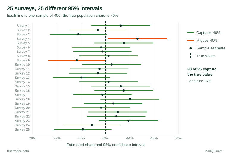
The key point is that the 95% belongs to the procedure, not to any single interval. Before a sample is drawn, there is a 95% chance that the interval about to be calculated will contain the true value. Once the sample has been drawn and the interval calculated, the true value is either inside it or not; in Neyman's framework the population value is fixed, not random, so no probability is attached to it (Neyman, 1937; Morey et al., 2016).
Figure 1 shows what this means. Each horizontal line is a 95% interval from a different hypothetical survey of the same population, in which the true share is 40%. Most intervals cross the true value, but a few miss. In real research we see only one of these lines and never know whether ours is one of the misses.
A worked example
Suppose a hypothetical telecoms survey interviews a simple random sample of 800 customers and finds that 272, or 34.0%, say they plan to switch provider in the next year. The standard error of a sample proportion p from a sample of size n is:
SE = √(p(1 − p) ÷ n) = √(0.34 × 0.66 ÷ 800) ≈ 0.0167
The 95% interval is 34.0% ± 1.96 × 1.67, or 34.0% ± 3.3 percentage points: 30.7% to 37.3%. A 99% interval is wider, 29.7% to 38.3%, because a method that succeeds more often has to cast a wider net.
A correct plain-language summary is: "Our best estimate is 34%. A range calculated this way would contain the true figure in 95% of surveys like this one, so the data are consistent with a true share of roughly 31% to 37%." Note what the summary does not say. It does not say there is a 95% probability that the true share lies between 30.7% and 37.3%, and it says nothing about errors other than sampling error.
Common misinterpretations
Hoekstra et al. (2014) gave researchers and students a confidence interval with six statements about it, all of which were false. Most participants, including experienced researchers, endorsed several of the false statements, and very few rejected them all. Greenland et al. (2016) catalogue similar errors in epidemiology and medicine. The following are the misreadings that do the most damage in applied work.
"There is a 95% probability that the true value is in this interval"
This is the most common misreading. In the frequentist framework that produces the interval, the 95% describes how often the method works across many samples, not the chance that a given interval is correct (Morey et al., 2016). In practice the distinction can seem subtle when there is little prior knowledge, but it becomes important when other information exists. If a firm already knows from billing data that churn has never exceeded 25% in any year, a survey interval of 30.7% to 37.3% does not carry a 95% chance of being right; it more likely signals bias in the survey. A statement of probability about the parameter needs a Bayesian analysis, discussed below.
"Values in the middle are much more likely; values near the ends are nearly ruled out"
Values near the point estimate are more compatible with the data than values near the limits, but the limits are not a cliff edge. A value just outside a 95% interval is barely less compatible with the data than a value just inside it. Greenland et al. (2016) and Amrhein et al. (2019) suggest calling intervals "compatibility intervals" for this reason, and warn against treating the limits as sharp boundaries between "possible" and "impossible".
"95% of the data lie within the interval"
A confidence interval describes uncertainty about a population value such as a mean, not the spread of individual observations. A 95% interval for the average customer spend of $42 ± $3 does not mean that most customers spend between $39 and $45. Individual spending may range from zero to hundreds of dollars. The range that covers a stated share of individuals is a prediction interval or tolerance interval, and it is much wider.
"If we repeat the survey, there is a 95% chance the new estimate will fall inside this interval"
This sounds natural but is wrong. Both the original interval and the new estimate are subject to sampling error, so the new estimate falls inside the old interval less often than 95% of the time. Cumming and Maillardet (2006) showed that, on average, a 95% interval captures the next sample's mean only about 83% of the time. Business users who expect a tracking survey to stay within last month's interval will see more "surprising" movements than they expect.
"Overlapping intervals mean there is no significant difference"
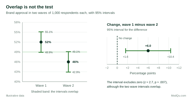
Two groups can have overlapping 95% intervals and still differ significantly at the 5% level. Checking for overlap is a conservative test: it misses many real differences (Schenker & Gentleman, 2001). Belia et al. (2005) found that many researchers, asked to position two means so that the difference was just significant, placed the intervals so that they barely touched, a far stricter standard than p = .05.
Figure 2 gives an example. In a hypothetical brand-tracking study of 1,000 respondents per wave, approval is 52% in one wave and 46% in the next. The intervals overlap, from 48.9% to 49.1%, but the interval for the difference runs from 1.6 to 10.4 points and excludes zero. The correct approach is to calculate the interval for the difference directly, because the standard error of a difference is smaller than the sum of the two separate standard errors.
"The interval includes zero, so there is no effect"
An interval for a difference that includes zero shows that the data are compatible with no effect, but also with every other value in the range. If a price-test interval for the change in conversion runs from −0.5 to +4.0 points, the data are as consistent with a sizeable gain as with no change. Amrhein et al. (2019) argue that reading such results as "no effect" is one of the most damaging habits in research. The width of the interval is the message: the study was too small to settle the question.
"A narrow interval means the estimate is accurate"
The interval reflects only random sampling error, under the assumptions of the method. It says nothing about coverage error, nonresponse bias, poorly worded questions or a wrong model (Kish, 1965; Lohr, 2021). A survey of 20,000 people from a biased online panel will produce a very narrow interval around a possibly wrong number. Precision and accuracy are different properties, and large samples improve only the first.
Confidence intervals and Bayesian credible intervals
If decision-makers want to say "there is a 95% probability that the true value lies between a and b", the appropriate tool is a Bayesian credible interval. Bayesian inference combines the data with a prior distribution that expresses what was believed before the study, and produces a posterior distribution for the parameter itself (Gelman et al., 2013). With large samples and weak priors, the two kinds of interval are often numerically close, which is one reason the misreading persists. With small samples, strong prior knowledge or constrained parameters, they can differ substantially, and Morey et al. (2016) give examples in which a confidence interval is clearly uninformative even though it has correct coverage. Neither approach is automatically better, but each should be described in its own terms.
Choosing the right interval
The textbook formula is not always the right one.
- Proportions near 0% or 100%, or small samples. The simple "Wald" interval used in the worked example performs poorly when the proportion is extreme or the sample small. Brown et al. (2001) showed that its actual coverage can fall well below 95%, even with samples in the hundreds, and fluctuates unpredictably with n. The Wilson (1927) score interval or the Agresti and Coull (1998) adjustment, which in effect adds two successes and two failures, perform much better. For 2 complaints among 40 customers (5%), the Wald interval runs from −1.8% to 11.8%, an impossible lower limit; the Wilson interval is 1.4% to 16.5%.
- Skewed data and complex statistics. For medians, ratios, percentiles or model outputs without a simple standard error, the bootstrap resamples the observed data many times to approximate the sampling distribution (Efron, 1979).
- Complex survey designs. Clustering, stratification and weighting change the standard error. Clustered and heavily weighted samples usually have wider intervals than the simple random sample formula suggests, which is captured by the design effect. Design-based standard errors should be used whenever the data come from such a design (Kish, 1965; Lohr, 2021).
Practical guidance for survey and business reports
- Always report an interval alongside the estimate. A point estimate on its own invites false precision. Intervals show both the best estimate and how much it could plausibly differ from the truth (Gardner & Altman, 1986; Cumming, 2014).
- Use one standard sentence. For example: "The best estimate is 34%; the data are consistent with values between 31% and 37%." Avoid "we are 95% sure the true value is…" in formal reporting.
- Compare groups with intervals for the difference, not by inspecting overlap. Cumming and Finch (2005) give rules of thumb for reading interval charts, but a direct calculation is clearer.
- Do not let the interval replace judgement. The American Statistical Association warns against reducing evidence to a single threshold (Wasserstein & Lazar, 2016). An interval that excludes zero is not proof of a meaningful effect, and one that includes zero is not proof of no effect.
- Beware of selected results. If a dashboard shows intervals for 40 segments and the reader focuses on the most extreme, the stated 95% coverage no longer applies to the selected ones. Benjamini and Yekutieli (2005) propose adjusted intervals for exactly this situation.
- Be cautious with small, noisy studies. When precision is low, the estimates that happen to reach significance tend to exaggerate the true effect and can even have the wrong sign (Gelman & Carlin, 2014).
- State what the interval leaves out. A short note that the interval reflects sampling error only, and not nonresponse or measurement problems, prevents over-confident readings.
Key takeaways
A 95% confidence interval comes from a method that captures the true value in 95% of repeated samples. It does not give a 95% probability that any one interval is correct, it does not describe the spread of individual data, and it does not predict where the next survey will land. Overlapping intervals do not rule out a real difference, and an interval that includes zero does not show that there is no effect. Intervals cover sampling error only, so a narrow interval from a biased sample can still be wrong. Used with these limits in mind, and with methods suited to the data, confidence intervals remain one of the clearest ways of showing decision-makers both what the data say and how firmly they say it.
References
Agresti, A., & Coull, B. A. (1998). Approximate is better than "exact" for interval estimation of binomial proportions. The American Statistician, 52(2), 119–126. https://doi.org/10.1080/00031305.1998.10480550
Amrhein, V., Greenland, S., & McShane, B. (2019). Scientists rise up against statistical significance. Nature, 567(7748), 305–307. https://doi.org/10.1038/d41586-019-00857-9
Belia, S., Fidler, F., Williams, J., & Cumming, G. (2005). Researchers misunderstand confidence intervals and standard error bars. Psychological Methods, 10(4), 389–396. https://doi.org/10.1037/1082-989X.10.4.389
Benjamini, Y., & Yekutieli, D. (2005). False discovery rate–adjusted multiple confidence intervals for selected parameters. Journal of the American Statistical Association, 100(469), 71–81. https://doi.org/10.1198/016214504000001907
Brown, L. D., Cai, T. T., & DasGupta, A. (2001). Interval estimation for a binomial proportion. Statistical Science, 16(2), 101–133. https://doi.org/10.1214/ss/1009213286
Casella, G., & Berger, R. L. (2002). Statistical inference (2nd ed.). Duxbury.
Cumming, G. (2014). The new statistics: Why and how. Psychological Science, 25(1), 7–29. https://doi.org/10.1177/0956797613504966
Cumming, G., & Finch, S. (2005). Inference by eye: Confidence intervals and how to read pictures of data. American Psychologist, 60(2), 170–180. https://doi.org/10.1037/0003-066X.60.2.170
Cumming, G., & Maillardet, R. (2006). Confidence intervals and replication: Where will the next mean fall? Psychological Methods, 11(3), 217–227. https://doi.org/10.1037/1082-989X.11.3.217
Efron, B. (1979). Bootstrap methods: Another look at the jackknife. The Annals of Statistics, 7(1), 1–26. https://doi.org/10.1214/aos/1176344552
Gardner, M. J., & Altman, D. G. (1986). Confidence intervals rather than P values: Estimation rather than hypothesis testing. British Medical Journal, 292(6522), 746–750. https://doi.org/10.1136/bmj.292.6522.746
Gelman, A., & Carlin, J. (2014). Beyond power calculations: Assessing Type S (sign) and Type M (magnitude) errors. Perspectives on Psychological Science, 9(6), 641–651. https://doi.org/10.1177/1745691614551642
Gelman, A., Carlin, J. B., Stern, H. S., Dunson, D. B., Vehtari, A., & Rubin, D. B. (2013). Bayesian data analysis (3rd ed.). Chapman and Hall/CRC. https://doi.org/10.1201/b16018
Greenland, S., Senn, S. J., Rothman, K. J., Carlin, J. B., Poole, C., Goodman, S. N., & Altman, D. G. (2016). Statistical tests, P values, confidence intervals, and power: A guide to misinterpretations. European Journal of Epidemiology, 31(4), 337–350. https://doi.org/10.1007/s10654-016-0149-3
Hoekstra, R., Morey, R. D., Rouder, J. N., & Wagenmakers, E.-J. (2014). Robust misinterpretation of confidence intervals. Psychonomic Bulletin & Review, 21(5), 1157–1164. https://doi.org/10.3758/s13423-013-0572-3
Kish, L. (1965). Survey sampling. Wiley.
Lohr, S. L. (2021). Sampling: Design and analysis (3rd ed.). Chapman and Hall/CRC. https://doi.org/10.1201/9780429298899
Morey, R. D., Hoekstra, R., Rouder, J. N., Lee, M. D., & Wagenmakers, E.-J. (2016). The fallacy of placing confidence in confidence intervals. Psychonomic Bulletin & Review, 23(1), 103–123. https://doi.org/10.3758/s13423-015-0947-8
Neyman, J. (1937). Outline of a theory of statistical estimation based on the classical theory of probability. Philosophical Transactions of the Royal Society of London. Series A, Mathematical and Physical Sciences, 236(767), 333–380. https://doi.org/10.1098/rsta.1937.0005
Schenker, N., & Gentleman, J. F. (2001). On judging the significance of differences by examining the overlap between confidence intervals. The American Statistician, 55(3), 182–186. https://doi.org/10.1198/000313001317097960
Wasserstein, R. L., & Lazar, N. A. (2016). The ASA statement on p-values: Context, process, and purpose. The American Statistician, 70(2), 129–133. https://doi.org/10.1080/00031305.2016.1154108
Wilson, E. B. (1927). Probable inference, the law of succession, and statistical inference. Journal of the American Statistical Association, 22(158), 209–212. https://doi.org/10.1080/01621459.1927.10502953