
Statistics · Tests and models
Hidden Markov Models for Latent State Sequence Knowledge
How hidden Markov models infer unobserved states such as customer engagement or economic regimes from sequences of observations, how they are estimated and decoded, and where they mislead.
Many of the things businesses care about cannot be observed directly. A customer is "engaged" or "drifting away"; an economy is in expansion or recession; a panel respondent is answering carefully or speeding through. What we do observe is a sequence of noisy signals: purchases, visits, growth figures, response times. A hidden Markov model (HMM) is a statistical model for exactly this situation. It assumes that an unobserved state evolves over time according to simple rules, and that each observation is generated by whichever state is active at that moment. From the observed sequence, the model works backwards to the most plausible sequence of hidden states.
The mathematical foundations were laid in the late 1960s (Baum & Petrie, 1966; Baum et al., 1970), and the models became famous through speech recognition, where the hidden states are sounds and the observations are acoustic measurements (Rabiner, 1989). They are now used in genetics, finance, ecology, psychology and marketing. This article explains how HMMs work, walks through a small worked example, and sets out practical guidance for applying them to survey panels and customer data.
The core idea: a hidden chain and visible signals
An HMM combines two simple parts. The first is a Markov chain of hidden states. At each time point the system is in one of K states, and the probability of moving to the next state depends only on the current state, not on the full history. This is the Markov property, and it is what keeps the model tractable. The second part is an emission (or state-dependent) distribution: given the current state, the observation is drawn from a distribution specific to that state. An engaged customer buys often; a disengaged customer buys rarely; but either may occasionally behave out of character.
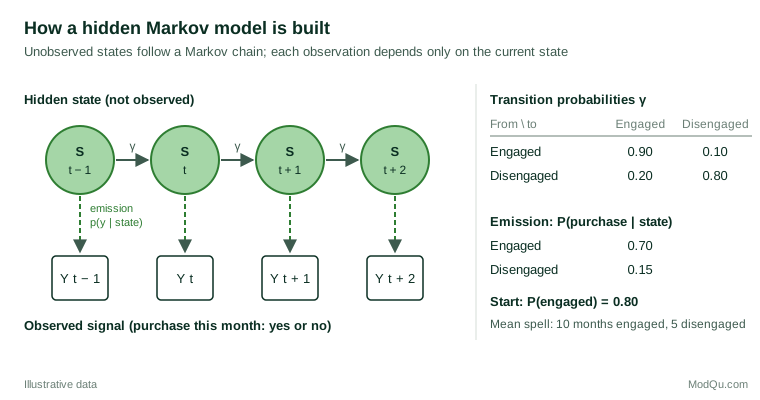
Formally, an HMM with hidden states S1, …, ST and observations Y1, …, YT is defined by three sets of parameters (Rabiner & Juang, 1986):
- Initial probabilities δi = P(S1 = i), the chance of starting in each state.
- Transition probabilities γij = P(St+1 = j | St = i), collected in a K × K matrix whose rows sum to 1.
- Emission distributions P(Yt = y | St = i), which may be Bernoulli for yes/no outcomes, Poisson for counts, normal for continuous measures, or multinomial for categorical answers.
The joint probability of a hidden path and the observed data is then a simple product:
P(s1:T, y1:T) = δs1 · ps1(y1) · ∏t=2T γst−1st · pst(yt)
Two useful quantities follow directly from the transition matrix. The expected time spent in state i before leaving is 1 ÷ (1 − γii), so a "stay" probability of 0.9 implies an average spell of ten periods. And the long-run share of time in each state is given by the chain's stationary distribution. In this sense an HMM is a dynamic version of a mixture model, or of latent class analysis: each observation belongs to an unobserved class, but class membership is allowed to change over time in a structured way (Zucchini et al., 2016; McLachlan & Peel, 2000).
Three questions an HMM answers
Rabiner's (1989) influential tutorial framed HMM analysis around three problems, and the framing remains the clearest way to understand what the models do.
1. How likely are these data? (Evaluation)
Given a set of parameters, what is the probability of the observed sequence? Summing over every possible hidden path is impossible for long sequences, because the number of paths grows as KT. The forward algorithm solves this by moving through time and keeping, for each state, the probability of the data so far and of being in that state now. The cost grows only linearly with the length of the sequence. The likelihood it produces is the basis for estimation and for comparing models.
2. Which states were active? (Decoding)
Two different answers are possible, and they are often confused. Local decoding asks, for each time point separately, which state is most probable given all the data. It uses the forward–backward algorithm, which combines a forward pass with a matching backward pass to give the smoothed probability of each state at each time. Global decoding asks for the single most probable complete sequence of states. It uses the Viterbi algorithm, a dynamic programming method originally developed for decoding signals in communication systems (Viterbi, 1967; Forney, 1973). The two answers usually agree, but not always: the sequence of individually most likely states is not necessarily the most likely sequence.
A related distinction matters for real-time use. Filtered probabilities use only data up to time t, which is what an analyst monitoring customers this month actually has. Smoothed probabilities use the whole sequence, including later months, and are more accurate for looking back.
3. What are the parameters? (Learning)
In practice the transition and emission probabilities are unknown and must be estimated from data. The standard approach is maximum likelihood using the Baum–Welch algorithm (Baum et al., 1970), which was later recognised as a special case of the expectation–maximisation (EM) algorithm (Dempster et al., 1977). It alternates between computing expected state memberships with the forward–backward algorithm and updating the parameters as if those memberships were known. Each cycle increases the likelihood, but the algorithm can stop at a local rather than a global maximum, so it should be run from many different starting values (Zucchini et al., 2016). The likelihood can also be maximised directly with numerical optimisers. Bayesian estimation, typically using Markov chain Monte Carlo, is a well-developed alternative that gives full uncertainty for the states and parameters (Scott, 2002; Frühwirth-Schnatter, 2006).
A worked example: tracking customer engagement
Consider a hypothetical subscription retailer that records, for one customer, whether a purchase was made in each of twelve months. The observed sequence is:
1, 1, 0, 1, 1, 0, 0, 0, 1, 0, 0, 0
We fit (or, for this illustration, assume) a two-state model with the parameters in Figure 1. Engaged customers buy in a given month with probability 0.70 and remain engaged next month with probability 0.90. Disengaged customers buy with probability 0.15, stay disengaged with probability 0.80, and return to engagement with probability 0.20. Customers start engaged with probability 0.80. These values imply average spells of ten months engaged and five months disengaged, and a long-run share of two-thirds of time in the engaged state.
Running the forward–backward and Viterbi algorithms on this sequence gives the results in Figure 2 and the table below (all values illustrative, computed exactly from the stated parameters).
| Month | Purchase | Filtered P(disengaged) | Smoothed P(disengaged) | Viterbi state |
|---|---|---|---|---|
| 3 | No | 0.28 | 0.13 | Engaged |
| 6 | No | 0.29 | 0.57 | Disengaged |
| 8 | No | 0.73 | 0.71 | Disengaged |
| 9 | Yes | 0.25 | 0.58 | Disengaged |
| 12 | No | 0.81 | 0.81 | Disengaged |
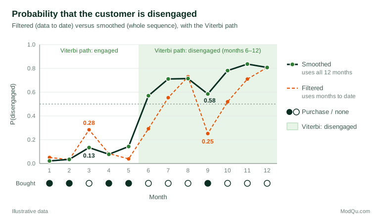
Three lessons stand out. First, the model is not fooled by a single quiet month: the missed purchase in month 3 raises the filtered probability of disengagement only to 0.28, and once the purchases in months 4 and 5 are taken into account, the smoothed probability falls to 0.13. A simple rule such as "flag any customer who did not buy last month" would have raised a false alarm. Second, the purchase in month 9 looks like a recovery in real time (the filtered probability falls to 0.25), but with hindsight the model judges it more likely to be an isolated purchase by a customer who remained disengaged (smoothed probability 0.58). Third, the Viterbi path places a single switch, from engaged to disengaged, at month 6. That is a clean story for a report, but it hides the uncertainty: in month 6 the probability of disengagement is only 0.57.
For a retention team, the practical output is the filtered probability, updated monthly, with a threshold chosen by weighing the cost of a retention offer against the value of a saved customer.
Where HMMs are used
Speech and language. HMMs dominated speech recognition for several decades, with states representing sounds within words (Rabiner, 1989).
Biology. Protein family modelling and gene finding use HMMs in which the hidden states are positions in a family of related sequences, or regions such as coding and non-coding DNA (Krogh et al., 1994; Eddy, 2004).
Economics and finance. Hamilton's (1989) Markov-switching model treated economic growth as switching between expansion and recession regimes, and dated recessions in United States output from the data alone. Regime-switching models of returns and volatility follow the same logic.
Marketing and customer analytics. Netzer et al. (2008) used an HMM to model the relationship between alumni and their university, with hidden relationship states driving the probability of giving. The same structure fits subscription, loyalty and churn data, where the hidden state is the strength of the customer relationship and the observations are transactions, visits or survey responses.
Survey and panel research. In longitudinal surveys, latent transition analysis applies the same ideas to repeated categorical answers, estimating how people move between unobserved classes such as attitudes or stages of change (Collins & Lanza, 2009). Markov latent class models are also used to separate real change in a panel from measurement error: if a respondent's reported status flips back and forth, some of that movement is probably misclassification rather than true change (Biemer, 2011). Within a single questionnaire, response times and answer patterns can be modelled as signals of hidden response styles, such as attentive and careless answering.
Practical guidance for business and survey data
Choose the number of states with care. There is no single correct test. Information criteria such as AIC (Akaike, 1974) and BIC (Schwarz, 1978) are widely used, and BIC is usually more conservative. With large data sets, however, both tend to favour more states than are useful, because they pick up minor features the model was not designed to capture. Pohle et al. (2017) recommend combining criteria with substantive judgement: start with the smallest number of states that answers the business question, inspect what each additional state represents, and check the fit with residual diagnostics.
Name states after their profiles, not your hopes. States are defined only by their emission distributions. A state labelled "loyal" should show the behaviour that word implies. Check that states are well separated; if two states have similar emission probabilities, the model cannot tell them apart reliably.
Add covariates where they matter. Transition probabilities can depend on covariates such as price changes, marketing contact or tenure, and emission probabilities can depend on observed characteristics. This turns a descriptive model into one that can test, for example, whether a service failure increases the chance of moving into disengagement. Software such as the depmixS4 package in R supports covariates on both parts of the model (Visser & Speekenbrink, 2010).
Use many sequences. One customer's twelve months cannot identify the parameters. Models are estimated on many sequences, often assuming that all customers share the same parameters. If segments behave differently, a mixture of HMMs or random effects can allow for it.
Think about time spacing. The basic model assumes equally spaced observations and a constant transition matrix. Irregular contact data, such as purchases recorded only when they happen, may need a continuous-time model or careful aggregation into periods.
Check the Markov assumption. The basic HMM implies that time spent in a state follows a geometric distribution: the chance of leaving does not depend on how long one has been there. In many settings, such as a new subscriber's honeymoon period, this is unrealistic. Semi-Markov models relax it at the cost of added complexity (Zucchini et al., 2016).
Common mistakes
- Reporting the Viterbi path as fact. The decoded sequence is an estimate. Report state probabilities alongside it, as in Figure 2.
- Using smoothed probabilities for real-time decisions. Smoothed values use future data that are not available when a decision is made. Evaluate any monitoring rule on filtered probabilities.
- Trusting a single estimation run. Baum–Welch can converge to a poor local optimum. Tutorials such as Visser (2011) stress multiple starting values. Watch also for label switching, where the meaning of "state 1" and "state 2" swaps between runs.
- Over-interpreting extra states. A model with five states will often fit better than one with three, but the extra states may only describe unusual months rather than distinct customer conditions.
- Ignoring survey design. When sequences come from a weighted panel, unweighted estimates describe the sample, not the population. Weights and attrition patterns should be considered when estimating population transition rates.
- Assuming the states are causes. A hidden state is a summary of a behaviour pattern. It does not by itself explain why customers move between states.
Model checking and validation
Fitted HMMs should be checked like any other model. Pseudo-residuals, which convert each observation into a value that should look normally distributed if the model is correct, are a standard diagnostic for both outliers and systematic misfit (Zucchini et al., 2016). Simulating sequences from the fitted model and comparing them with the real data, for example on run lengths or the share of months with purchases, is a direct test of whether the model reproduces the patterns that matter. For predictive uses such as churn warning, hold out later months and compare the model's forecasts with what actually happened. Theoretical results on consistency and asymptotic behaviour of estimators are reviewed by Cappé et al. (2005); in applied work, the parametric bootstrap is a practical way to obtain standard errors.
Key takeaways
A hidden Markov model treats an observed sequence as noisy evidence about an unobserved state that changes over time. It is defined by initial, transition and emission probabilities, estimated by the Baum–Welch (EM) algorithm or Bayesian methods, and decoded with the forward–backward and Viterbi algorithms. For business and survey analysts, its main strength is distinguishing lasting shifts from one-off fluctuations: a single quiet month need not signal churn, and a single purchase need not signal recovery. Use HMMs with many sequences, a small and interpretable number of states, multiple starting values, filtered probabilities for real-time decisions, and clear reporting of uncertainty in the decoded states.
References
Akaike, H. (1974). A new look at the statistical model identification. IEEE Transactions on Automatic Control, 19(6), 716–723. https://doi.org/10.1109/TAC.1974.1100705
Baum, L. E., & Petrie, T. (1966). Statistical inference for probabilistic functions of finite state Markov chains. The Annals of Mathematical Statistics, 37(6), 1554–1563. https://doi.org/10.1214/aoms/1177699147
Baum, L. E., Petrie, T., Soules, G., & Weiss, N. (1970). A maximization technique occurring in the statistical analysis of probabilistic functions of Markov chains. The Annals of Mathematical Statistics, 41(1), 164–171. https://doi.org/10.1214/aoms/1177697196
Biemer, P. P. (2011). Latent class analysis of survey error. Wiley. https://doi.org/10.1002/9780470891155
Cappé, O., Moulines, E., & Rydén, T. (2005). Inference in hidden Markov models. Springer. https://doi.org/10.1007/0-387-28982-8
Collins, L. M., & Lanza, S. T. (2009). Latent class and latent transition analysis: With applications in the social, behavioral, and health sciences. Wiley. https://doi.org/10.1002/9780470567333
Dempster, A. P., Laird, N. M., & Rubin, D. B. (1977). Maximum likelihood from incomplete data via the EM algorithm. Journal of the Royal Statistical Society Series B: Statistical Methodology, 39(1), 1–22. https://doi.org/10.1111/j.2517-6161.1977.tb01600.x
Eddy, S. R. (2004). What is a hidden Markov model? Nature Biotechnology, 22(10), 1315–1316. https://doi.org/10.1038/nbt1004-1315
Forney, G. D., Jr. (1973). The Viterbi algorithm. Proceedings of the IEEE, 61(3), 268–278. https://doi.org/10.1109/PROC.1973.9030
Frühwirth-Schnatter, S. (2006). Finite mixture and Markov switching models. Springer. https://doi.org/10.1007/978-0-387-35768-3
Hamilton, J. D. (1989). A new approach to the economic analysis of nonstationary time series and the business cycle. Econometrica, 57(2), 357–384. https://doi.org/10.2307/1912559
Krogh, A., Brown, M., Mian, I. S., Sjölander, K., & Haussler, D. (1994). Hidden Markov models in computational biology: Applications to protein modeling. Journal of Molecular Biology, 235(5), 1501–1531. https://doi.org/10.1006/jmbi.1994.1104
McLachlan, G., & Peel, D. (2000). Finite mixture models. Wiley. https://doi.org/10.1002/0471721182
Netzer, O., Lattin, J. M., & Srinivasan, V. (2008). A hidden Markov model of customer relationship dynamics. Marketing Science, 27(2), 185–204. https://doi.org/10.1287/mksc.1070.0294
Pohle, J., Langrock, R., van Beest, F. M., & Schmidt, N. M. (2017). Selecting the number of states in hidden Markov models: Pragmatic solutions illustrated using animal movement. Journal of Agricultural, Biological and Environmental Statistics, 22(3), 270–293. https://doi.org/10.1007/s13253-017-0283-8
Rabiner, L. R. (1989). A tutorial on hidden Markov models and selected applications in speech recognition. Proceedings of the IEEE, 77(2), 257–286. https://doi.org/10.1109/5.18626
Rabiner, L. R., & Juang, B. H. (1986). An introduction to hidden Markov models. IEEE ASSP Magazine, 3(1), 4–16. https://doi.org/10.1109/MASSP.1986.1165342
Schwarz, G. (1978). Estimating the dimension of a model. The Annals of Statistics, 6(2), 461–464. https://doi.org/10.1214/aos/1176344136
Scott, S. L. (2002). Bayesian methods for hidden Markov models: Recursive computing in the 21st century. Journal of the American Statistical Association, 97(457), 337–351. https://doi.org/10.1198/016214502753479464
Visser, I. (2011). Seven things to remember about hidden Markov models: A tutorial on Markovian models for time series. Journal of Mathematical Psychology, 55(6), 403–415. https://doi.org/10.1016/j.jmp.2011.08.002
Visser, I., & Speekenbrink, M. (2010). depmixS4: An R package for hidden Markov models. Journal of Statistical Software, 36(7), 1–21. https://doi.org/10.18637/jss.v036.i07
Viterbi, A. (1967). Error bounds for convolutional codes and an asymptotically optimum decoding algorithm. IEEE Transactions on Information Theory, 13(2), 260–269. https://doi.org/10.1109/TIT.1967.1054010
Zucchini, W., MacDonald, I. L., & Langrock, R. (2016). Hidden Markov models for time series: An introduction using R (2nd ed.). Chapman and Hall/CRC. https://doi.org/10.1201/b20790