
Statistics · Tests and models
Functional Data Analysis for Curve and Trajectory Knowledge
How functional data analysis treats each customer journey, tracking series or growth path as a single curve, and how smoothing and functional principal components reveal the shapes that matter.
Some business data are not really a list of separate numbers. A customer's monthly spend over the first year, a brand's weekly awareness score, the load on a website across a day or a respondent's dial-turn ratings during an advertisement are each better seen as one smooth curve sampled at many points. Functional data analysis (FDA) is the branch of statistics that treats each such curve, rather than each measurement, as the unit of analysis (Ramsay & Silverman, 2005). It asks questions about shape: when growth levels off, which customers peak early and fade, and how whole trajectories differ between segments.
Curves as data
Classical multivariate methods treat twelve monthly values as twelve variables. That approach ignores the order of the months, struggles when people are measured at different times and wastes the information that neighbouring values are similar. FDA instead assumes that behind the noisy observations for each unit lies a smooth function xi(t), and it analyses those functions directly (Ramsay & Dalzell, 1991). Once data are curves, derivatives become available too: the slope of a spend curve is a rate of growth, and its curvature shows acceleration or slowdown.
Typical candidates in market research include continuous tracking studies, moment-by-moment ratings collected while respondents watch an advertisement, usage logs that record activity every day, and repeated survey waves in which the same people are interviewed several times. In each case the interesting questions concern the whole path: how quickly a score recovers after a negative news story, whether two segments follow the same life-cycle shape, or how long the effect of a campaign lasts before fading.
Reviews by Wang et al. (2016) and Kokoszka and Reimherr (2017) describe the field's main tools. Three of them do most of the work in practice: smoothing, functional principal component analysis and functional regression.
Step 1: smoothing raw observations into curves
Each unit's observations are turned into a function by combining a set of basis functions, usually B-splines for non-periodic data or Fourier terms for seasonal data:
xi(t) = ci1φ1(t) + ci2φ2(t) + … + ciKφK(t)
A roughness penalty stops the curve from chasing every random fluctuation. Penalised splines (Eilers & Marx, 1996) offer a convenient, stable way to do this, with the amount of smoothing chosen by generalised cross-validation. The aim is a curve that keeps genuine features, such as a seasonal peak, while discarding measurement error.
When curves are sparse, with only a handful of irregular observations per person, as in many panel surveys, smoothing each curve separately fails. Yao et al. (2005) showed how to pool information across all units to estimate the mean and covariance, then recover each person's curve from very few points.
Step 2: functional principal components
Functional principal component analysis (FPCA) is the functional version of principal component analysis. It finds a small number of shapes, called eigenfunctions, that describe how curves depart from the mean curve. Each curve can then be written approximately as:
xi(t) ≈ μ(t) + ξi1ψ1(t) + ξi2ψ2(t)
Here μ(t) is the mean curve, ψ1 and ψ2 are the leading modes of variation and the scores ξi1 and ξi2 say how strongly each unit expresses them. The scores are ordinary numbers that can be used in cluster analysis, regression or dashboards.
A worked example
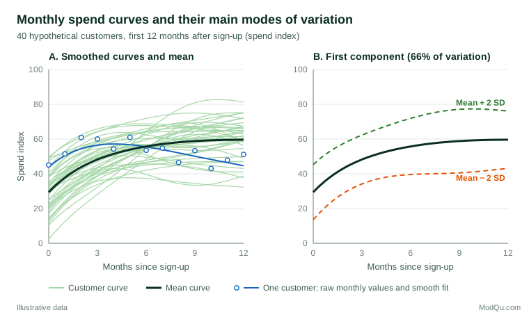
Consider a hypothetical subscription business that tracks a monthly spend index for 40 new customers over their first 12 months (Figure 1). The raw values for any one customer are jumpy, as the blue points show, but the smoothed curve captures the underlying pattern: a rise over the first few months and then a gradual decline.
FPCA on these curves gives two clear components. The first explains about 66% of the variation and acts mainly as an overall level: customers with high scores spend more throughout the year. The second explains about 32% and contrasts early and late months, separating customers who start strongly and fade from those who build slowly. Together they account for almost all of the variation, so each customer's year can be summarised by two scores. A customer with an average level but a strongly negative second score is an early-fade customer and a natural target for retention offers in month four or five, before the decline is visible in a quarterly report.
Functional regression and other extensions
Functional regression links curves to other variables (Morris, 2015). In a scalar-on-function model, a single outcome such as twelve-month retention is predicted from a whole curve, such as the first three months of usage. In a function-on-scalar model, a whole curve, such as an awareness trajectory, is explained by covariates such as region or campaign exposure. Ferraty and Vieu (2006) developed nonparametric versions, and Horváth and Kokoszka (2012) provide hypothesis tests for comparing groups of curves and for functional time series.
FDA also supports forecasting. Hyndman and Ullah (2007) forecast entire age-specific mortality and fertility curves by modelling functional principal component scores over time, an approach that transfers well to forecasting a full daily demand profile rather than a single total.
Practical guidance for survey and business data
- Choose a sensible time axis. Align curves by sign-up date, campaign launch or customer age rather than calendar date when the question is about life-cycle shape.
- Separate amplitude from timing. Two customers can have the same peak at different times. Registration, or curve alignment, distinguishes variation in height from variation in timing (Marron et al., 2015).
- Check the smoothing. Plot raw points over fitted curves for a sample of units. Over-smoothing hides real turning points; under-smoothing turns noise into apparent structure.
- Use established software. The methods in Ramsay et al. (2009) are implemented in freely available packages, which reduces the risk of coding errors.
- Account for sample design. If the units come from a weighted survey, apply weights when estimating the mean curve and covariance.
Limitations and common mistakes
- Treating dense noise as signal. Smooth curves look precise, but they are estimates. Report confidence bands, not only fitted lines.
- Over-reading components. Eigenfunctions are mathematical summaries, not behavioural types. Name them carefully and check that the interpretation holds on new data.
- Ignoring sparse or irregular sampling. Interpolating a few points per person and then running ordinary FPCA can produce distorted components; use methods designed for sparse data.
- Assuming causation. A link between early-usage curves and retention does not show that changing early usage would change retention.
Key takeaways
Functional data analysis is the right tool when each unit's data are best thought of as a curve. Smoothing turns noisy observations into functions, functional principal components reduce whole trajectories to a few interpretable scores and functional regression connects curves to outcomes. For tracking studies, customer life cycles and any repeated measurement over time, FDA turns many columns of numbers into a clear account of shape, timing and change.
References
Eilers, P. H. C., & Marx, B. D. (1996). Flexible smoothing with B-splines and penalties. Statistical Science, 11(2), 89–121. https://doi.org/10.1214/ss/1038425655
Ferraty, F., & Vieu, P. (2006). Nonparametric functional data analysis: Theory and practice. Springer. https://doi.org/10.1007/0-387-36620-2
Horváth, L., & Kokoszka, P. (2012). Inference for functional data with applications. Springer. https://doi.org/10.1007/978-1-4614-3655-3
Hyndman, R. J., & Ullah, M. S. (2007). Robust forecasting of mortality and fertility rates: A functional data approach. Computational Statistics & Data Analysis, 51(10), 4942–4956. https://doi.org/10.1016/j.csda.2006.07.028
Kokoszka, P., & Reimherr, M. (2017). Introduction to functional data analysis. Chapman and Hall/CRC. https://doi.org/10.1201/9781315117416
Marron, J. S., Ramsay, J. O., Sangalli, L. M., & Srivastava, A. (2015). Functional data analysis of amplitude and phase variation. Statistical Science, 30(4), 468–484. https://doi.org/10.1214/15-STS524
Morris, J. S. (2015). Functional regression. Annual Review of Statistics and Its Application, 2(1), 321–359. https://doi.org/10.1146/annurev-statistics-010814-020413
Ramsay, J. O., & Dalzell, C. J. (1991). Some tools for functional data analysis. Journal of the Royal Statistical Society Series B: Statistical Methodology, 53(3), 539–561. https://doi.org/10.1111/j.2517-6161.1991.tb01844.x
Ramsay, J. O., Hooker, G., & Graves, S. (2009). Functional data analysis with R and MATLAB. Springer. https://doi.org/10.1007/978-0-387-98185-7
Ramsay, J. O., & Silverman, B. W. (2005). Functional data analysis (2nd ed.). Springer. https://doi.org/10.1007/b98888
Wang, J.-L., Chiou, J.-M., & Müller, H.-G. (2016). Functional data analysis. Annual Review of Statistics and Its Application, 3(1), 257–295. https://doi.org/10.1146/annurev-statistics-041715-033624
Yao, F., Müller, H.-G., & Wang, J.-L. (2005). Functional data analysis for sparse longitudinal data. Journal of the American Statistical Association, 100(470), 577–590. https://doi.org/10.1198/016214504000001745