
Statistics · Data science and machine learning
Ensemble Methods and Model Averaging for Robust Knowledge Aggregation
How bagging, random forests, boosting, stacking and forecast combination pool many imperfect models into more accurate and stable predictions, and what that pooling can and cannot tell us.
A single statistical model is one view of the data, shaped by its assumptions, its sample and the choices of the analyst who built it. Ensemble methods combine many such views. Instead of searching for the one best model, they fit several and pool their predictions. The idea is old in forecasting, where Bates and Granger (1969) showed that a combination of two airline passenger forecasts could be more accurate than either alone, and it is now central to predictive modelling, where tree ensembles are among the most accurate general-purpose methods available (Hastie et al., 2009).
This article explains the main ensemble methods, why averaging works, and what analysts of survey and business data should keep in mind when using them. Bayesian model averaging, which weights models by their posterior probability, is covered in a separate article; the focus here is on bagging, random forests, boosting, stacking and forecast combination.
Why averaging helps
Suppose B models each make prediction errors with the same variance σ², and the errors of any two models have correlation ρ. The variance of their average is (Hastie et al., 2009):
Var(average) = ρσ² + (1 − ρ)σ² ÷ B
As more models are added, the second term shrinks towards zero, but the first does not. Averaging removes the part of the error that the models do not share; it cannot remove the part they do. The left panel of Figure 1 shows the consequence. With uncorrelated errors, averaging 50 models cuts the variance by 98%. With a correlation of 0.75, it cuts it by only about 25%, however many models are added.
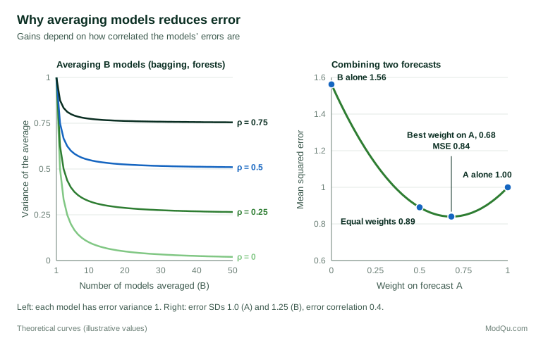
The lesson is that ensembles gain most from members that are individually reasonable but different from one another. Dietterich (2000) gives three reasons why a combination can outperform its best member: with limited data, many models fit equally well and averaging reduces the risk of choosing a poor one; fitting algorithms can get stuck in different local solutions; and a combination can represent patterns that no single member can.
Bagging and random forests
Decision trees are flexible but unstable: a small change in the data can produce a very different tree. Breiman (1996) proposed bagging (bootstrap aggregating) to exploit this instability. Many bootstrap samples are drawn from the data, a tree is grown on each, and the predictions are averaged, or put to a majority vote for classification. Each tree is noisy, but their noise partly cancels.
Because the bootstrap samples overlap heavily, bagged trees remain quite similar, so ρ stays high. Random forests reduce it by also choosing a random subset of predictors as candidates at each split (Breiman, 2001). Strong predictors can no longer dominate every tree, so the trees differ more and their average is more stable. Each tree is also tested on the observations left out of its bootstrap sample, giving an "out-of-bag" error estimate without a separate validation set.
Random forests need little tuning and handle many predictors, interactions and non-linear effects. They are a strong default for tasks such as predicting churn from survey and behavioural data. Their variable importance measures need care, however: Strobl et al. (2007) showed that the standard measures can favour continuous predictors and categorical predictors with many levels, even when these are no more relevant.
Boosting
Bagging builds models independently and averages them. Boosting builds them in sequence, with each new model concentrating on what the previous ones got wrong. In AdaBoost, observations that were misclassified receive more weight in the next round (Freund & Schapire, 1997). Friedman et al. (2000) showed that this procedure can be understood as fitting an additive model in stages, which connected boosting to familiar statistical ideas.
Friedman (2001) generalised the approach as gradient boosting. Each new tree is fitted to the residuals, or more generally to the gradient of a chosen loss function, and added to the ensemble with a small weight, the learning rate. Small learning rates and many trees usually generalise better than large steps. Efficient implementations such as XGBoost made gradient boosting fast enough for very large datasets (Chen & Guestrin, 2016), and boosted trees are now among the most accurate methods for tabular business data.
Where bagging mainly reduces variance, boosting mainly reduces bias, by building a complex model from many simple ones. The price is a greater risk of overfitting: the number of trees, their depth and the learning rate should be tuned by cross-validation.
Stacking
Stacking, or stacked generalisation, combines models of different kinds (Wolpert, 1992). Several base models, such as a logistic regression, a random forest and a boosted model, each produce predictions. A second-level model then learns how best to combine them. To avoid rewarding overfitted members, the second-level model is trained on cross-validated predictions, made for each observation by base models that did not see it. This approach was later formalised as the super learner, which in large samples performs essentially as well as the best weighted combination of the candidate models (van der Laan et al., 2007).
Forecast combination
In business forecasting, combining forecasts from different methods or different experts has a long and successful record. Clemen (1989), reviewing a large body of studies, concluded that combining forecasts reliably improves accuracy and that simple averages often perform as well as more elaborate weighting schemes. Timmermann (2006) reached similar conclusions in a later review. In the M4 competition, which compared forecasting methods on 100,000 time series, combinations of methods were among the most accurate approaches (Makridakis et al., 2020).
The right panel of Figure 1 shows why combining helps even when one forecaster is clearly better. Forecast A has a mean squared error of 1.00 and forecast B of 1.56. The optimal combination puts a weight of 0.68 on A and reduces the error to 0.84. A simple equal-weight average, which ignores the fact that A is better, still achieves 0.89, beating both individual forecasts.
That the simple average so often rivals optimal weights in practice is known as the forecast combination puzzle. Smith and Wallis (2009) explain it as a result of estimation error: optimal weights must be estimated from limited past data, and the noise in those estimates can cost more than the theoretical gain. When forecasters are of similar quality, or when the track record is short, equal weights are usually the safer choice.
Ensembles as knowledge aggregation
The same logic applies beyond algorithms. A market research team that combines a survey-based demand estimate, a time-series forecast from sales records and the judgement of regional managers is building an ensemble. The combination is most valuable when the sources are informed by different evidence, because their errors are then least correlated. It is least valuable when everyone reads the same report, uses the same data or defers to the same senior opinion, which pushes the correlation towards one. This is the statistical basis of the wisdom of crowds: independence and diversity of judgement matter more than the number of judges.
Ensembles also carry a lesson about uncertainty. When members disagree sharply, the average hides real doubt about the answer. Reporting the spread of member predictions alongside the combined forecast tells decision-makers how much the evidence agrees.
Practical guidance and limitations
- Diversity matters more than number. Adding near-copies of the same model adds little. Combine methods that use different assumptions, predictors or data.
- Validate the whole ensemble. Tune and evaluate on data not used for fitting, and use cross-validated predictions for stacking.
- Prefer simple weights when evidence is thin. Estimated combination weights need long track records to beat an equal-weight average.
- Ensembles do not fix biased data. If every member is trained on the same unrepresentative sample or flawed outcome measure, they share the error, and averaging cannot remove it. In terms of the formula above, shared bias acts like a correlation of one.
- Interpretation is harder. A forest of 500 trees has no single set of coefficients. Use variable importance and partial dependence plots with care, and keep a simpler model alongside for explanation when stakeholders need to understand the drivers.
- Combine probabilities, not just labels. For classification, averaging predicted probabilities usually works better than majority voting, and the resulting probabilities should be checked for calibration.
- Respect survey structure. Bootstrap samples and cross-validation folds should respect clustering and weighting where these affect the target population.
Key takeaways
Ensemble methods turn many imperfect models into one more reliable predictor. Bagging and random forests average unstable trees to reduce variance; boosting adds models in sequence to reduce bias; stacking learns how to weight different kinds of model; and forecast combination pools independent forecasts, often most robustly with equal weights. All rely on the same principle: errors that models do not share cancel when they are averaged, while errors they do share remain. Ensembles therefore aggregate knowledge best when their members are diverse, and they can never correct a bias that every member has learned from the same data.
References
Bates, J. M., & Granger, C. W. J. (1969). The combination of forecasts. Operational Research Quarterly, 20(4), 451–468. https://doi.org/10.1057/jors.1969.103
Breiman, L. (1996). Bagging predictors. Machine Learning, 24(2), 123–140. https://doi.org/10.1007/BF00058655
Breiman, L. (2001). Random forests. Machine Learning, 45(1), 5–32. https://doi.org/10.1023/A:1010933404324
Chen, T., & Guestrin, C. (2016). XGBoost: A scalable tree boosting system. In Proceedings of the 22nd ACM SIGKDD International Conference on Knowledge Discovery and Data Mining (pp. 785–794). ACM. https://doi.org/10.1145/2939672.2939785
Clemen, R. T. (1989). Combining forecasts: A review and annotated bibliography. International Journal of Forecasting, 5(4), 559–583. https://doi.org/10.1016/0169-2070(89)90012-5
Dietterich, T. G. (2000). Ensemble methods in machine learning. In Multiple Classifier Systems: First International Workshop, MCS 2000 (Lecture Notes in Computer Science, Vol. 1857, pp. 1–15). Springer. https://doi.org/10.1007/3-540-45014-9_1
Freund, Y., & Schapire, R. E. (1997). A decision-theoretic generalization of on-line learning and an application to boosting. Journal of Computer and System Sciences, 55(1), 119–139. https://doi.org/10.1006/jcss.1997.1504
Friedman, J. H. (2001). Greedy function approximation: A gradient boosting machine. The Annals of Statistics, 29(5), 1189–1232. https://doi.org/10.1214/aos/1013203451
Friedman, J., Hastie, T., & Tibshirani, R. (2000). Additive logistic regression: A statistical view of boosting (with discussion and a rejoinder by the authors). The Annals of Statistics, 28(2), 337–407. https://doi.org/10.1214/aos/1016218223
Hastie, T., Tibshirani, R., & Friedman, J. (2009). The elements of statistical learning: Data mining, inference, and prediction (2nd ed.). Springer. https://doi.org/10.1007/978-0-387-84858-7
Makridakis, S., Spiliotis, E., & Assimakopoulos, V. (2020). The M4 Competition: 100,000 time series and 61 forecasting methods. International Journal of Forecasting, 36(1), 54–74. https://doi.org/10.1016/j.ijforecast.2019.04.014
Smith, J., & Wallis, K. F. (2009). A simple explanation of the forecast combination puzzle. Oxford Bulletin of Economics and Statistics, 71(3), 331–355. https://doi.org/10.1111/j.1468-0084.2008.00541.x
Strobl, C., Boulesteix, A.-L., Zeileis, A., & Hothorn, T. (2007). Bias in random forest variable importance measures: Illustrations, sources and a solution. BMC Bioinformatics, 8(1), Article 25. https://doi.org/10.1186/1471-2105-8-25
Timmermann, A. (2006). Forecast combinations. In G. Elliott, C. W. J. Granger, & A. Timmermann (Eds.), Handbook of economic forecasting (Vol. 1, pp. 135–196). Elsevier. https://doi.org/10.1016/S1574-0706(05)01004-9
van der Laan, M. J., Polley, E. C., & Hubbard, A. E. (2007). Super learner. Statistical Applications in Genetics and Molecular Biology, 6(1), Article 25. https://doi.org/10.2202/1544-6115.1309
Wolpert, D. H. (1992). Stacked generalization. Neural Networks, 5(2), 241–259. https://doi.org/10.1016/S0893-6080(05)80023-1