
Statistics · Data science and machine learning
Penalized Regression (Lasso, Ridge, Elastic Net) for High-Dimensional Knowledge
How ridge, lasso and elastic net regression add a penalty to keep models with many predictors stable and predictive, how to tune them, and what they can and cannot tell decision-makers.
Modern business data sets are wide. A customer survey may carry 80 attitude items, and a text-mining step can create thousands of word counts for every respondent. When the number of candidate predictors approaches or exceeds the number of observations, ordinary least squares regression stops working well. Coefficients swing wildly from sample to sample, the model fits the noise in the training data, and predictions for new customers are poor. Penalized regression is the standard family of remedies. It adds a cost for large coefficients to the usual fitting criterion, trading a small, deliberate bias for a large reduction in variance. Three members of the family dominate practice: ridge regression, the lasso and the elastic net.
This article explains how each method works, how to choose the amount of penalty, and where the methods' limits lie, especially when analysts want to read selected variables as the "true drivers" of an outcome.
The problem: too many predictors, too little information
Ordinary least squares (OLS) chooses the coefficients that minimise the sum of squared residuals. With a modest number of well-separated predictors and a reasonable sample, OLS is unbiased and efficient. Two features of modern data undermine it.
The first is collinearity. Survey items often measure overlapping ideas: satisfaction with "service", "support" and "staff friendliness" may correlate at 0.8 or more. When predictors are highly correlated, the data contain little information about their separate effects, so OLS estimates have very large variances. Hoerl and Kennard (1970) described this as the problem of "nonorthogonal" predictors and showed that the least squares estimates are, on average, too long: their squared length is inflated by noise.
The second is dimensionality. When the number of predictors p is close to the sample size n, OLS fits the training data almost perfectly and generalises badly, a textbook case of overfitting. When p exceeds n, OLS has no unique solution at all. Stepwise and best-subset selection search over subsets of predictors, but the search is discrete: a variable is either in or out. Breiman (1995) showed that such procedures are unstable, in the sense that small changes in the data can produce a very different chosen model and noticeably different predictions.
Penalized regression replaces this discrete search with a continuous one. Instead of asking which variables to include, it asks how far each coefficient should be pulled towards zero.
The general idea: fit plus penalty
All three methods minimise a criterion of the same form:
Σi (yi − β0 − Σj xijβj)2 + λ × P(β)
The first term is the familiar residual sum of squares. The second term, P(β), measures the size of the coefficient vector, and the tuning parameter λ ≥ 0 controls how heavily size is punished. When λ = 0 the method reduces to OLS. As λ grows, coefficients shrink towards zero, the model becomes simpler, and its variance falls while its bias rises. The best predictive model usually lies somewhere in between, and finding it is the main practical task (Hastie et al., 2009).
Two conventions matter before fitting. Predictors are almost always standardised to mean zero and standard deviation one, because the penalty treats all coefficients alike: without standardisation, a variable measured in dollars would be penalised differently from the same variable measured in thousands of dollars. The intercept β0 is not penalised. The widely used glmnet software does both by default (Friedman et al., 2010).
The same logic extends beyond linear regression. Adding a penalty to the log-likelihood gives penalized logistic regression for yes/no outcomes such as churn, penalized Poisson regression for counts and penalized Cox models for time-to-event data; in other words, penalties can be attached to any generalised linear model (Friedman et al., 2010; Hastie et al., 2015).
Ridge regression: shrink everything a little
Ridge regression uses the squared length of the coefficient vector as its penalty, known as the L2 penalty:
P(β) = Σj βj2
Hoerl and Kennard (1970) proposed ridge regression to deal with collinearity and proved that there is always some positive value of the penalty for which the ridge estimator has smaller mean squared error than OLS. The ridge solution has a closed form, (X′X + λI)−1X′y, and adding λ to the diagonal of X′X makes the matrix invertible even when predictors are perfectly collinear or p exceeds n.
Ridge regression shrinks all coefficients smoothly and proportionally more in directions of the data that carry little information. It never sets a coefficient exactly to zero. With strongly correlated predictors, ridge tends to share the effect among them rather than choosing one, which usually makes predictions more stable. That is a strength when many predictors each carry a little signal, such as hundreds of browsing variables that each contribute weakly to purchase propensity, and a weakness when the analyst wants a short list of variables to report.
The lasso: shrinkage and selection together
Tibshirani (1996) introduced the lasso (least absolute shrinkage and selection operator), which replaces the squared penalty with the sum of absolute values, the L1 penalty:
P(β) = Σj |βj|
This apparently small change has a striking consequence. Because the absolute-value function has a corner at zero, the lasso sets some coefficients exactly to zero once λ is large enough. It therefore performs shrinkage and variable selection in a single, continuous procedure. Geometrically, the lasso constraint region is a diamond (in two dimensions) with corners on the axes, while the ridge region is a circle; the elliptical contours of the residual sum of squares often first touch the diamond at a corner, where one coefficient is zero (Tibshirani, 1996; James et al., 2021).
Frank and Friedman (1993) had already considered "bridge" penalties of the form Σ|βj|q; ridge corresponds to q = 2 and the lasso to q = 1, the smallest value that still gives a convex, computationally convenient problem. Breiman's (1995) non-negative garrote, a related idea, also shrinks and selects but starts from the OLS estimates.
Efficient algorithms made the lasso practical. Least angle regression computes the entire lasso solution path, for every value of λ, at roughly the cost of a single least squares fit (Efron et al., 2004). Coordinate descent, implemented in glmnet, is faster still and handles logistic and multinomial outcomes with tens of thousands of predictors (Friedman et al., 2010).
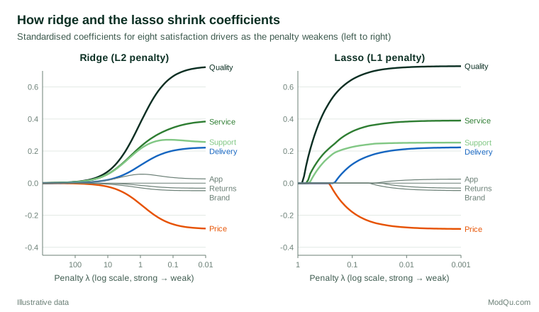
In Figure 1, under a strong penalty the lasso keeps only Quality; as the penalty weakens, Service, Support, Price and Delivery enter in turn, and the three predictors with no true effect enter last with tiny coefficients. Ridge gives every predictor a non-zero coefficient at every penalty level.
Known weaknesses of the lasso
The lasso has three well-documented limitations. First, when p exceeds n, it can select at most n variables before it saturates. Second, from a group of highly correlated predictors it tends to pick one more or less arbitrarily and ignore the rest (Zou & Hastie, 2005). Third, the same penalty that selects variables also shrinks the coefficients of the variables it keeps, so large true effects are biased towards zero, and the lasso does not always identify the correct set of variables even with large samples. Zou (2006) showed that the lasso can be inconsistent for variable selection in some settings and proposed the adaptive lasso, which uses weights so that large coefficients are penalised less. Fan and Li (2001) proposed a non-convex penalty, SCAD, with similar aims. Both have "oracle" properties: under regularity conditions, they perform asymptotically as well as if the true predictors were known in advance. The theory of when the lasso can recover the true model, including the conditions on correlations among predictors that this requires, is set out in detail by Bühlmann and van de Geer (2011).
The elastic net: a compromise
Zou and Hastie (2005) proposed the elastic net to combine the strengths of both penalties. Its penalty is a weighted mix:
P(β) = α Σj |βj| + (1 − α) ÷ 2 × Σj βj2
The mixing parameter α runs from 0 (pure ridge) to 1 (pure lasso); this is the parameterisation used in glmnet (Friedman et al., 2010). The L1 part still produces exact zeros, so the elastic net selects variables. The L2 part stabilises the solution and creates what Zou and Hastie (2005) called a grouping effect: strongly correlated predictors tend to enter or leave the model together, with similar coefficients. The elastic net can also select more than n variables when p exceeds n. For survey batteries in which several items measure the same underlying attitude, this behaviour is often more sensible than the lasso's arbitrary choice of a single item.
The group lasso applies the penalty to predefined groups of coefficients so that a whole group enters or leaves together (Yuan & Lin, 2006). This suits categorical predictors coded as several dummy variables, such as region, where keeping some categories and dropping others makes little sense.
| Method | Penalty | Sets coefficients to zero? | Correlated predictors | Typical use |
|---|---|---|---|---|
| Ridge | Sum of squares (L2) | No | Shares the effect among them | Prediction with many weak signals |
| Lasso | Sum of absolute values (L1) | Yes | Tends to pick one | Sparse, interpretable prediction models |
| Elastic net | Mix of L1 and L2 | Yes | Selects them as a group | Wide data with correlated blocks |
Choosing the penalty: cross-validation
The amount of penalty, λ (and α for the elastic net), is not estimated from the fitting criterion itself, because the criterion always prefers λ = 0. It is chosen to optimise predictive accuracy on data not used for fitting, almost always by K-fold cross-validation (Stone, 1974). The data are split into K folds, often 5 or 10. For each candidate λ, the model is fitted on K − 1 folds and its prediction error is measured on the held-out fold; the errors are then averaged over the folds.
Two choices of λ are common. The value with the lowest cross-validated error, often written λmin, gives the best estimated predictive accuracy. The one-standard-error rule instead selects the largest λ whose error is within one standard error of the minimum, giving a simpler model whose accuracy cannot be distinguished from the best (Hastie et al., 2009; James et al., 2021).
A worked example
Consider a hypothetical study in which 150 respondents rate a new service and the analyst has 120 candidate predictors: demographic variables, past purchase measures and attitude items. Only eight of them truly affect the rating. With p this close to n, OLS would fit the training data almost perfectly and predict poorly. Figure 2 shows ten-fold cross-validation for the lasso over a grid of 60 penalty values.
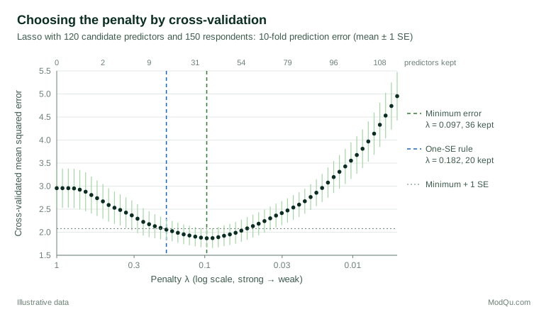
The curve has the U shape typical of the bias–variance trade-off. With a very strong penalty, the model keeps no predictors and simply predicts the mean, so the error is high (about 2.95). As the penalty weakens, the eight real effects enter and error falls to a minimum of about 1.87 at λ = 0.097, where 36 predictors are kept. With a weak penalty, more than 100 predictors are kept, the model chases noise and the error rises to almost 5. The one-standard-error rule picks λ = 0.182 and keeps 20 predictors. In this illustrative run, both choices retain all eight true predictors; the λmin model simply also carries 28 noise variables with small coefficients, and the one-standard-error model carries 12. The lasso tuned for prediction commonly includes too many variables rather than too few, which matters if the list will be presented as drivers.
Cross-validation pitfalls
Three mistakes are frequent in applied work.
- Reporting the tuning error as the final error. The minimum of the cross-validation curve is an optimistic estimate of future performance, because λ was chosen to make it small. Varma and Simon (2006) showed that this bias can be large in wide data sets and recommended nested cross-validation, in which an outer loop estimates error and an inner loop tunes λ.
- Doing preparation outside the loop. Screening variables by their correlation with the outcome, imputing missing values or standardising using the full data, and then cross-validating only the final fit, leaks information from the test folds. Every data-dependent step must be repeated inside each fold (Hastie et al., 2009).
- Ignoring instability. A different random split into folds can change the chosen λ and the selected variables; repeat the cross-validation and average.
Interpreting penalized models
Prediction versus explanation
Shmueli (2010) distinguishes models built to explain (to estimate causal or structural effects) from models built to predict, and argues that the two goals call for different choices. Penalized regression is first and foremost a prediction tool. Its coefficients are deliberately biased towards zero, so they should not be read as unbiased estimates of effect sizes, and the absence of a variable from a lasso model does not show that it has no effect. A variable may be dropped because a correlated variable carries the same information, as with Service and Support in Figure 1.
Inference after selection
A tempting shortcut is to run the lasso, keep the selected variables, refit OLS on them and report the usual standard errors and p-values. This is not valid. The same data were used to choose the model and to test it, so conventional confidence intervals are too narrow and p-values too small. Berk et al. (2013) developed confidence intervals that remain valid whatever selection procedure was used, at the cost of being wider. Lockhart et al. (2014) proposed a covariance test for whether each variable entering the lasso path adds real signal. Where the goal is the effect of one specific variable, such as an advertising exposure, in the presence of many possible confounders, the post-double-selection approach of Belloni et al. (2014) uses the lasso twice, once for the outcome and once for the exposure, and then estimates the effect with ordinary regression on the union of selected controls. This gives valid confidence intervals under sparsity assumptions.
How stable is the selected set?
Stability selection offers a practical check on which variables are reliably chosen. The lasso is fitted repeatedly on random half-samples, and only variables selected in a high proportion of runs are reported (Meinshausen & Bühlmann, 2010). Meinshausen and Bühlmann showed that this approach bounds the expected number of falsely selected variables, which gives a business audience a clear statement of how much confidence the list deserves.
Is the lasso better than best subsets?
The answer depends on the signal-to-noise ratio. In a large simulation study, Hastie et al. (2020) found that best-subset selection tended to predict better when the signal-to-noise ratio was high, while the lasso did better when it was low, and the relaxed lasso, which reduces the shrinkage of selected coefficients, performed well across settings. Survey and behavioural data are typically noisy.
Practical guidance for survey and business data
- Decide the goal first. If the aim is the most accurate churn or purchase prediction, ridge or the elastic net with α around 0.5 is often a strong default. If the aim is a short, readable scorecard, the lasso or elastic net with the one-standard-error rule is more suitable.
- Prepare predictors carefully. Standardise continuous variables, consider the group lasso for multi-category factors, and decide whether Likert items are numeric scores or categories.
- Impute missing data within each training fold, not once on the whole file.
- Respect the survey design where it matters. Most software supports observation weights, so survey weights can be passed to the fit, but cross-validation folds should respect clustering (for example, keep all respondents from one household or one interviewer in the same fold).
- Use the right loss. For yes/no outcomes, fit penalized logistic regression and tune on deviance or the Brier score rather than raw accuracy, especially when the outcome is rare.
- Validate on new data. Hold out a recent wave or a separate region as a final test, and check calibration as well as discrimination. Harrell (2015) gives detailed guidance on validating and presenting shrunken prediction models.
- Expect variability in small samples. Shrinkage is meant to protect small studies from overfitting, but the tuned penalty itself is estimated with error. Van Calster et al. (2020) found in simulations that ridge and lasso improved calibration on average yet did not guarantee better performance in any single small data set, because the chosen penalty varied a great deal between samples. Planning an adequate sample size, rather than relying on penalization alone, remains the first line of defence.
Common mistakes
- Forgetting to standardise, so that the penalty depends on arbitrary units of measurement.
- Treating the selected variables as causes or as the complete set of drivers.
- Reporting naive p-values after selection, which overstates certainty.
- Comparing coefficient magnitudes across models with different penalties, since shrinkage depends on λ and on which other variables are present.
- Using penalization to rescue a hopelessly small sample.
Key takeaways
Ridge regression shrinks all coefficients and handles collinearity well but keeps every predictor. The lasso shrinks and selects in one step but behaves erratically with correlated predictors. The elastic net mixes the two and keeps correlated groups together. Choose the penalty by cross-validation, with every preparation step inside the loop and a separate estimate of final error. These methods make prediction from wide survey and customer data feasible even when predictors outnumber respondents. They are not, by themselves, tools for causal explanation or formal inference about which variables matter; for those goals, use post-selection methods, stability checks and careful study design (Hastie et al., 2015; Bühlmann & van de Geer, 2011).
References
Belloni, A., Chernozhukov, V., & Hansen, C. (2014). Inference on treatment effects after selection among high-dimensional controls. The Review of Economic Studies, 81(2), 608–650. https://doi.org/10.1093/restud/rdt044
Berk, R., Brown, L., Buja, A., Zhang, K., & Zhao, L. (2013). Valid post-selection inference. The Annals of Statistics, 41(2), 802–837. https://doi.org/10.1214/12-AOS1077
Breiman, L. (1995). Better subset regression using the nonnegative garrote. Technometrics, 37(4), 373–384. https://doi.org/10.1080/00401706.1995.10484371
Bühlmann, P., & van de Geer, S. (2011). Statistics for high-dimensional data: Methods, theory and applications. Springer. https://doi.org/10.1007/978-3-642-20192-9
Efron, B., Hastie, T., Johnstone, I., & Tibshirani, R. (2004). Least angle regression. The Annals of Statistics, 32(2), 407–499. https://doi.org/10.1214/009053604000000067
Fan, J., & Li, R. (2001). Variable selection via nonconcave penalized likelihood and its oracle properties. Journal of the American Statistical Association, 96(456), 1348–1360. https://doi.org/10.1198/016214501753382273
Frank, I. E., & Friedman, J. H. (1993). A statistical view of some chemometrics regression tools. Technometrics, 35(2), 109–135. https://doi.org/10.1080/00401706.1993.10485033
Friedman, J., Hastie, T., & Tibshirani, R. (2010). Regularization paths for generalized linear models via coordinate descent. Journal of Statistical Software, 33(1), 1–22. https://doi.org/10.18637/jss.v033.i01
Harrell, F. E., Jr. (2015). Regression modeling strategies: With applications to linear models, logistic and ordinal regression, and survival analysis (2nd ed.). Springer. https://doi.org/10.1007/978-3-319-19425-7
Hastie, T., Tibshirani, R., & Friedman, J. (2009). The elements of statistical learning: Data mining, inference, and prediction (2nd ed.). Springer. https://doi.org/10.1007/978-0-387-84858-7
Hastie, T., Tibshirani, R., & Tibshirani, R. (2020). Best subset, forward stepwise or lasso? Analysis and recommendations based on extensive comparisons. Statistical Science, 35(4), 579–592. https://doi.org/10.1214/19-STS733
Hastie, T., Tibshirani, R., & Wainwright, M. (2015). Statistical learning with sparsity: The lasso and generalizations. Chapman and Hall/CRC. https://doi.org/10.1201/b18401
Hoerl, A. E., & Kennard, R. W. (1970). Ridge regression: Biased estimation for nonorthogonal problems. Technometrics, 12(1), 55–67. https://doi.org/10.1080/00401706.1970.10488634
James, G., Witten, D., Hastie, T., & Tibshirani, R. (2021). An introduction to statistical learning: With applications in R (2nd ed.). Springer. https://doi.org/10.1007/978-1-0716-1418-1
Lockhart, R., Taylor, J., Tibshirani, R. J., & Tibshirani, R. (2014). A significance test for the lasso. The Annals of Statistics, 42(2), 413–468. https://doi.org/10.1214/13-AOS1175
Meinshausen, N., & Bühlmann, P. (2010). Stability selection. Journal of the Royal Statistical Society Series B: Statistical Methodology, 72(4), 417–473. https://doi.org/10.1111/j.1467-9868.2010.00740.x
Shmueli, G. (2010). To explain or to predict? Statistical Science, 25(3), 289–310. https://doi.org/10.1214/10-STS330
Stone, M. (1974). Cross-validatory choice and assessment of statistical predictions. Journal of the Royal Statistical Society Series B: Statistical Methodology, 36(2), 111–133. https://doi.org/10.1111/j.2517-6161.1974.tb00994.x
Tibshirani, R. (1996). Regression shrinkage and selection via the lasso. Journal of the Royal Statistical Society Series B: Statistical Methodology, 58(1), 267–288. https://doi.org/10.1111/j.2517-6161.1996.tb02080.x
Van Calster, B., van Smeden, M., De Cock, B., & Steyerberg, E. W. (2020). Regression shrinkage methods for clinical prediction models do not guarantee improved performance: Simulation study. Statistical Methods in Medical Research, 29(11), 3166–3178. https://doi.org/10.1177/0962280220921415
Varma, S., & Simon, R. (2006). Bias in error estimation when using cross-validation for model selection. BMC Bioinformatics, 7, Article 91. https://doi.org/10.1186/1471-2105-7-91
Yuan, M., & Lin, Y. (2006). Model selection and estimation in regression with grouped variables. Journal of the Royal Statistical Society Series B: Statistical Methodology, 68(1), 49–67. https://doi.org/10.1111/j.1467-9868.2005.00532.x
Zou, H. (2006). The adaptive lasso and its oracle properties. Journal of the American Statistical Association, 101(476), 1418–1429. https://doi.org/10.1198/016214506000000735
Zou, H., & Hastie, T. (2005). Regularization and variable selection via the elastic net. Journal of the Royal Statistical Society Series B: Statistical Methodology, 67(2), 301–320. https://doi.org/10.1111/j.1467-9868.2005.00503.x