
Statistics · Data science and machine learning
Model Selection Criteria (AIC, BIC, Cross-Validation) and Their Epistemic Implications
How AIC, BIC and cross-validation choose between competing models, what each assumes about truth and prediction, and why the choice of criterion shapes what an analysis can honestly claim.
Almost every statistical analysis involves choosing a model. Which drivers belong in a regression of customer satisfaction? How many segments does a market contain? Should a sales forecast include last year's seasonal pattern, a trend, or both? The data rarely answer these questions on their own, because a more complex model will always fit the data in hand at least as well as a simpler one. Model selection criteria exist to correct for that advantage, so that complexity is accepted only when it earns its place.
The three most widely used tools are the Akaike information criterion (AIC), the Bayesian information criterion (BIC) and cross-validation. They often agree. When they disagree, the disagreement is not a technical glitch: each criterion answers a different question, rests on different assumptions about what a model is for and implies a different view of what the resulting knowledge means. This article explains how each works, shows where they diverge and draws out the epistemic implications for analysts who report findings from survey and business data.
The problem: fit always improves
Adding a parameter to a model can only improve, or leave unchanged, its fit to the data used to estimate it. A regression with 20 predictors will have a higher R² than one with 5, even if the extra 15 are random noise. The extra flexibility lets the model fit the quirks of the particular sample, a problem known as overfitting. The fitted model then predicts new data less well than its training fit suggests.
Freedman (1983) gave a striking demonstration. He generated data in which the outcome was unrelated to any of 50 candidate predictors, screened the predictors for significance, refitted the model with those that passed, and obtained a highly significant overall result. Pure noise, after a little selection, looked like a discovery. Any honest selection procedure must therefore judge a model by something other than its fit to the data that chose it.
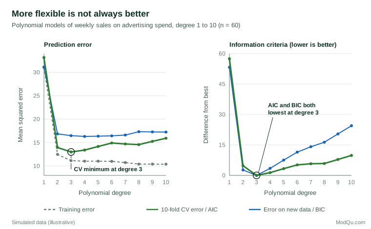
Figure 1 shows the pattern in a hypothetical example: weekly sales regressed on advertising spend using polynomial curves of increasing flexibility. Training error falls steadily as the degree rises. Error estimated by cross-validation, and error measured on a large set of new data, fall at first and then rise. The best model for prediction lies in between.
Akaike's information criterion
Akaike (1974) proposed judging a model by how close it is likely to come to the true process that generated the data, measured by the Kullback–Leibler divergence, an information-theoretic distance between probability distributions. He showed that the maximised log-likelihood of a model overstates its expected closeness to the truth by approximately the number of estimated parameters. Correcting for this gives:
AIC = −2 log L + 2k
where L is the maximised likelihood and k the number of estimated parameters. Lower values are better. The penalty of 2 per parameter is not arbitrary; it is the expected optimism of the fit. In small samples the approximation is poor, and Hurvich and Tsai (1989) derived a corrected version, AICc, which adds a further 2k(k + 1) ÷ (n − k − 1) and is recommended when the sample is small relative to the number of parameters.
AIC differences are interpreted on a relative scale. Burnham and Anderson (2002) suggest that models within about 2 units of the best have substantial support, models 4 to 7 units worse have considerably less, and models more than 10 units worse have essentially none. They also define Akaike weights, exp(−Δ/2) normalised to sum to one across the candidate models, which can be read as the relative support for each model given the data and the set of candidates.
The Bayesian information criterion
Schwarz (1978) approached the problem from a Bayesian angle. If one of the candidate models is true and each is given equal prior probability, the model with the highest posterior probability is the one with the largest marginal likelihood. For large samples this is approximated by:
BIC = −2 log L + k × ln(n)
The penalty per parameter is now the natural logarithm of the sample size. With n = 8 the two penalties are similar; with n = 1,000 each parameter costs about 6.9 units rather than 2, so BIC favours smaller models. Differences in BIC approximate twice the log of a Bayes factor, and Kass and Raftery (1995) give a scale for reading them: differences of 2 to 6 are positive evidence, 6 to 10 strong and above 10 very strong.
BIC has a property AIC lacks. If the true model is among the candidates, the probability that BIC selects it approaches one as the sample grows. Statisticians call this consistency. AIC, by contrast, keeps a fixed chance of including unnecessary parameters however large the sample becomes.
Cross-validation
Cross-validation takes a direct, empirical route (Stone, 1974). The data are split into K parts, or folds. Each model is fitted K times, each time leaving out one fold and measuring prediction error on it. The average error across folds estimates how well the model would predict new data from the same population. Leave-one-out cross-validation is the extreme case in which each fold contains a single observation.
Cross-validation makes few assumptions. It does not require a likelihood, so it can compare a regression with a decision tree or a neural network, and it can use whatever loss matters to the business, such as absolute error in units sold. Hastie et al. (2009) and James et al. (2021) recommend 5 or 10 folds as a good balance between bias and variance in the error estimate, and suggest a "one-standard-error rule": choose the simplest model whose cross-validated error is within one standard error of the minimum. Arlot and Celisse (2010) review the many variants and their properties.
Cross-validation's freedom from modelling assumptions comes at a price. It assumes that the held-out folds resemble the data the model will face in use, so that error on one random slice of the sample is a fair guide to error on the next customer, store or month. When the sample is unrepresentative, or the future differs from the past, cross-validation measures how well a model predicts more of the same data, not how well it will perform in a changed world. Its estimates also vary from one random split to another, so repeating the procedure with different splits is good practice.
How the three are related
The criteria are less different than they first appear. Stone (1977) proved that, for large samples, choosing a model by leave-one-out cross-validation is equivalent to choosing it by AIC. Both aim at predictive accuracy for new observations like the old ones. Shao (1993) showed that leave-one-out cross-validation shares AIC's lack of consistency for linear models, and that consistency requires leaving out a large and growing share of the data in each split, which makes cross-validation behave more like BIC.
Figure 2 shows the consequences in a simulation. The true model contains three predictors with effects of 1.0, 0.5 and 0.25 (residual standard deviation 1.5), and three further candidates have no effect. In each of 400 simulated datasets per sample size, all 64 possible combinations are compared.
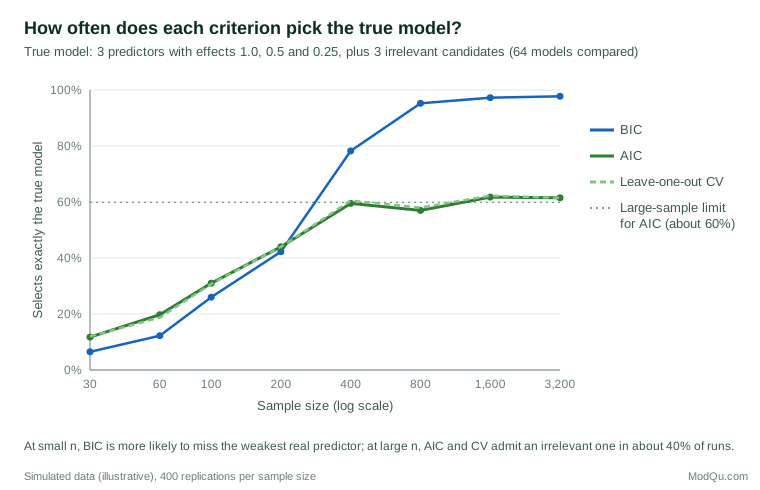
Three lessons follow. First, AIC and leave-one-out cross-validation track each other almost exactly, as Stone's result predicts. Second, in large samples BIC almost always finds the true model, whereas AIC still adds at least one irrelevant predictor in about 40% of datasets. The limiting figure can be calculated: AIC admits each irrelevant predictor with probability of about 16%, so the chance of admitting none of three is about 0.84³ ≈ 60%. Third, in small samples the ranking reverses. BIC's heavier penalty makes it more likely to leave out the weak but real predictor, and for prediction a slightly overfitted model often does better than one that misses a real effect.
Yang (2005) proved that this tension cannot be fully resolved: no selection rule can be both consistent, like BIC, and optimal for prediction error in the way AIC is. The analyst must decide which property matters more.
A worked example: drivers of recommendation
A hypothetical survey of 800 customers measures likelihood to recommend a service and several candidate drivers. Five nested regression models are compared. The table shows each model's maximised log-likelihood, number of parameters (including the intercept and residual variance), AIC, BIC and the resulting weights.
| Model | Log L | k | AIC | ΔAIC | AIC weight | BIC | ΔBIC | BIC weight |
|---|---|---|---|---|---|---|---|---|
| Price | −1,700.0 | 3 | 3,406.0 | 119.0 | 0.000 | 3,420.1 | 106.6 | 0.000 |
| + Service | −1,650.0 | 4 | 3,308.0 | 21.0 | 0.000 | 3,326.7 | 13.3 | 0.001 |
| + Ease of use | −1,640.0 | 5 | 3,290.0 | 3.0 | 0.122 | 3,313.4 | 0.0 | 0.698 |
| + Ad recall | −1,637.5 | 6 | 3,287.0 | 0.0 | 0.547 | 3,315.1 | 1.7 | 0.301 |
| + Region (3 terms) | −1,635.0 | 9 | 3,288.0 | 1.0 | 0.331 | 3,330.2 | 16.7 | 0.000 |
Both criteria agree that price, service and ease of use matter. They disagree about advertising recall. AIC prefers the model that includes it, while BIC prefers the model without it, though not decisively: a BIC difference of 1.7 is weak evidence by the Kass and Raftery (1995) scale. AIC also gives the model with region a third of the weight, while BIC rules it out. A 10-fold cross-validation would be expected to side broadly with AIC, given Stone's (1977) result.
What should be reported? Not simply "the best model includes advertising recall". A more honest summary is that three drivers are well supported, advertising recall improves prediction slightly but the evidence that it has a real effect is weak, and regional differences are unlikely to matter. That summary reflects the uncertainty in the selection itself, which a single "winning" model hides.
Epistemic implications
The choice of criterion is not only technical. Each embodies a view of what models are and what an analysis can claim to know.
Truth or usefulness?
BIC's derivation assumes that one candidate is the true model and seeks to identify it. AIC and cross-validation make no such assumption; they ask which model will predict best, accepting that all candidates are approximations. Burnham and Anderson (2004) argue that in the social and biological sciences the true process is far more complex than any candidate, so the premise behind BIC rarely holds. Box (1976) made the same point about models generally: the aim is to be usefully, not literally, correct.
The distinction matters for interpretation. A variable selected by BIC in a large sample has a reasonable claim to being a genuine part of the data-generating process, if the model family is right. A variable selected by AIC is better described as one that helps prediction. Shmueli (2010) argues that explaining and predicting are distinct goals that call for different modelling choices, and that confusing them is a common source of error. A driver analysis meant to guide investment is an explanatory claim; a churn model meant to rank customers is a predictive one.
Why prefer simpler models?
Philosophers have long debated why simplicity should count in favour of a theory. Forster and Sober (1994) used Akaike's result to give one answer: simpler models are not more likely to be true, but they are expected to predict more accurately when data are limited, because they are less prone to fitting noise. On this view the penalty for parameters is an estimate of overfitting, not a reward for elegance. As the sample grows, the case for simplicity weakens, which is why AIC's preferred model becomes more complex as data accumulate.
Selection is part of the inference
Once a model has been chosen, it is tempting to report its coefficients, standard errors and p-values as if it had been specified in advance. This ignores the selection step. Leeb and Pötscher (2005) showed that the sampling properties of estimates after model selection can differ sharply from those of the same estimates in a fixed model, and that confidence intervals computed in the usual way can badly overstate precision. Freedman's (1983) noise example is an extreme case of the same problem.
The same applies to cross-validation. If cross-validation is used both to choose a model and to report its expected error, the reported error is optimistic. Varma and Simon (2006) found that this bias can be substantial and recommended nested cross-validation, in which an outer loop estimates the performance of the whole selection procedure.
Many good models
Breiman (2001) described what he called the Rashomon effect: many quite different models may fit the data almost equally well while telling different stories about which variables matter. The worked example shows a mild version. Choosing one model and interpreting its coefficients treats an arbitrary choice among near-equivalents as a finding. Model averaging, whether by Akaike weights (Burnham & Anderson, 2002) or Bayesian model averaging (Hoeting et al., 1999), reports the spread of conclusions instead of hiding it.
The question shapes the answer
Claeskens and Hjort (2008) argue that the best model depends on the purpose. Their focused information criterion selects the model that best estimates the particular quantity of interest, which may differ from the one that best predicts the outcome overall. A model chosen to forecast total demand may not be the best for estimating the effect of a price change. Selection criteria answer the question they are built for, and the analyst should make sure it is the question being asked.
Practical guidance for survey and business data
- Decide the goal first. Use AIC or cross-validation when prediction is the aim; consider BIC when the aim is to identify which effects are real and the sample is large.
- Use AICc in small samples. When n ÷ k is below about 40, Burnham and Anderson (2002) recommend AICc over AIC.
- Respect the data structure in cross-validation. Random folds assume observations are exchangeable. For time series, hold out later periods; for panel or grouped data, hold out whole respondents, stores or regions (Roberts et al., 2017).
- Compare likelihood-based criteria only on the same data. AIC and BIC values are meaningless across different samples or different transformations of the outcome.
- Account for survey design. Standard AIC and BIC assume independent observations. With weights and clustering, design-based versions or cross-validation that respects clusters are safer.
- Report the candidate set and the weights. Show which models were considered and how strongly each was supported, as in the table above.
- Use nested cross-validation to report the expected performance of a model chosen by cross-validation.
- For Bayesian models, use approximate leave-one-out cross-validation or the widely applicable information criterion (WAIC), which use the full posterior rather than a point estimate (Vehtari et al., 2017).
Common mistakes
- Treating the selected model as true. Selection criteria rank the candidates offered; they cannot find a better model that was never considered.
- Reading AIC weights as probabilities that a model is true. They describe relative predictive support within the candidate set.
- Ignoring selection when reporting uncertainty. Post-selection standard errors and p-values are usually too small.
- Mixing criteria opportunistically. Choosing AIC for one question and BIC for another, depending on which gives the preferred answer, is a form of p-hacking.
- Cross-validating on time-ordered data with random folds. Future information leaks into the training data, and errors look smaller than they will be in practice.
Key takeaways
AIC, BIC and cross-validation all guard against overfitting, but they answer different questions. AIC and cross-validation estimate predictive accuracy and treat models as approximations; BIC seeks the true model and assumes it is among the candidates. In large samples BIC is consistent while AIC tends to keep extra terms; in small samples the opposite risk dominates. Because selection is itself an inference, honest reporting includes the candidate models, their relative support and the uncertainty that remains after choosing. The criterion an analyst chooses is, in effect, a statement about what kind of knowledge the analysis is meant to produce.
References
Akaike, H. (1974). A new look at the statistical model identification. IEEE Transactions on Automatic Control, 19(6), 716–723. https://doi.org/10.1109/TAC.1974.1100705
Arlot, S., & Celisse, A. (2010). A survey of cross-validation procedures for model selection. Statistics Surveys, 4, 40–79. https://doi.org/10.1214/09-SS054
Box, G. E. P. (1976). Science and statistics. Journal of the American Statistical Association, 71(356), 791–799. https://doi.org/10.1080/01621459.1976.10480949
Breiman, L. (2001). Statistical modeling: The two cultures (with comments and a rejoinder by the author). Statistical Science, 16(3), 199–231. https://doi.org/10.1214/ss/1009213726
Burnham, K. P., & Anderson, D. R. (2002). Model selection and multimodel inference: A practical information-theoretic approach (2nd ed.). Springer. https://doi.org/10.1007/b97636
Burnham, K. P., & Anderson, D. R. (2004). Multimodel inference: Understanding AIC and BIC in model selection. Sociological Methods & Research, 33(2), 261–304. https://doi.org/10.1177/0049124104268644
Claeskens, G., & Hjort, N. L. (2008). Model selection and model averaging. Cambridge University Press. https://doi.org/10.1017/CBO9780511790485
Forster, M., & Sober, E. (1994). How to tell when simpler, more unified, or less ad hoc theories will provide more accurate predictions. The British Journal for the Philosophy of Science, 45(1), 1–35. https://doi.org/10.1093/bjps/45.1.1
Freedman, D. A. (1983). A note on screening regression equations. The American Statistician, 37(2), 152–155. https://doi.org/10.1080/00031305.1983.10482729
Hastie, T., Tibshirani, R., & Friedman, J. (2009). The elements of statistical learning: Data mining, inference, and prediction (2nd ed.). Springer. https://doi.org/10.1007/978-0-387-84858-7
Hoeting, J. A., Madigan, D., Raftery, A. E., & Volinsky, C. T. (1999). Bayesian model averaging: A tutorial. Statistical Science, 14(4), 382–417. https://doi.org/10.1214/ss/1009212519
Hurvich, C. M., & Tsai, C.-L. (1989). Regression and time series model selection in small samples. Biometrika, 76(2), 297–307. https://doi.org/10.1093/biomet/76.2.297
James, G., Witten, D., Hastie, T., & Tibshirani, R. (2021). An introduction to statistical learning: With applications in R (2nd ed.). Springer. https://doi.org/10.1007/978-1-0716-1418-1
Kass, R. E., & Raftery, A. E. (1995). Bayes factors. Journal of the American Statistical Association, 90(430), 773–795. https://doi.org/10.1080/01621459.1995.10476572
Leeb, H., & Pötscher, B. M. (2005). Model selection and inference: Facts and fiction. Econometric Theory, 21(1), 21–59. https://doi.org/10.1017/S0266466605050036
Roberts, D. R., Bahn, V., Ciuti, S., Boyce, M. S., Elith, J., Guillera-Arroita, G., Hauenstein, S., Lahoz-Monfort, J. J., Schröder, B., Thuiller, W., Warton, D. I., Wintle, B. A., Hartig, F., & Dormann, C. F. (2017). Cross-validation strategies for data with temporal, spatial, hierarchical, or phylogenetic structure. Ecography, 40(8), 913–929. https://doi.org/10.1111/ecog.02881
Schwarz, G. (1978). Estimating the dimension of a model. The Annals of Statistics, 6(2), 461–464. https://doi.org/10.1214/aos/1176344136
Shao, J. (1993). Linear model selection by cross-validation. Journal of the American Statistical Association, 88(422), 486–494. https://doi.org/10.1080/01621459.1993.10476299
Shmueli, G. (2010). To explain or to predict? Statistical Science, 25(3), 289–310. https://doi.org/10.1214/10-STS330
Stone, M. (1974). Cross-validatory choice and assessment of statistical predictions. Journal of the Royal Statistical Society Series B: Statistical Methodology, 36(2), 111–133. https://doi.org/10.1111/j.2517-6161.1974.tb00994.x
Stone, M. (1977). An asymptotic equivalence of choice of model by cross-validation and Akaike's criterion. Journal of the Royal Statistical Society Series B: Statistical Methodology, 39(1), 44–47. https://doi.org/10.1111/j.2517-6161.1977.tb01603.x
Varma, S., & Simon, R. (2006). Bias in error estimation when using cross-validation for model selection. BMC Bioinformatics, 7, Article 91. https://doi.org/10.1186/1471-2105-7-91
Vehtari, A., Gelman, A., & Gabry, J. (2017). Practical Bayesian model evaluation using leave-one-out cross-validation and WAIC. Statistics and Computing, 27(5), 1413–1432. https://doi.org/10.1007/s11222-016-9696-4
Yang, Y. (2005). Can the strengths of AIC and BIC be shared? A conflict between model identification and regression estimation. Biometrika, 92(4), 937–950. https://doi.org/10.1093/biomet/92.4.937