
Statistics · Data science and machine learning
Anomaly Detection in Business Data
How to find unusual values in sales, transactions, operations and survey data, from robust statistical rules and control charts to isolation forests, and how to separate real signals from errors and false alarms.
A sudden spike in refunds, a store whose sales fall on its busiest day, an expense claim three times larger than any other, a survey respondent who completes a 20-minute questionnaire in three minutes. Each is an anomaly: an observation that does not fit the pattern of the rest of the data. Hawkins (1980) gave the classic definition of an outlier as an observation that deviates so much from the others that it arouses suspicion it was generated by a different mechanism.
Anomalies matter in business for two opposite reasons. Some are errors, such as duplicated records, wrong units or broken data feeds, and they distort every average, trend and model built on the data. Others are the most valuable signals in the data: fraud, equipment failure, a pricing mistake, a competitor's move or a sudden change in customer behaviour. Anomaly detection is the set of methods for finding both, so that people can decide which is which.
Three kinds of anomaly
Chandola et al. (2009), in a widely cited survey, distinguish three types:
- Point anomalies: a single value that is unusual compared with all others, such as a $48,000 transaction on an account whose purchases are usually under $200.
- Contextual anomalies: a value that is unusual only in its context. 104 orders is normal on a Tuesday but alarming on a Saturday; heating costs that would be normal in January are anomalous in July.
- Collective anomalies: a group of values that is unusual together although each looks normal alone, such as a run of identical answers in a survey grid or a sequence of small card payments that together form a fraud pattern.
Which type is being sought determines which method is appropriate. Simple rules find point anomalies; contextual anomalies need a model of what is expected in each context; collective anomalies need methods that look at sequences or groups.
Simple rules and why they fail
The most common rule flags any value more than three standard deviations from the mean. It has a serious weakness called masking: the anomalies themselves inflate the mean and standard deviation, which makes them look less unusual (Rousseeuw & Hubert, 2011).
Consider ten hypothetical weekly refund totals, in thousands of dollars: 12, 14, 13, 15, 11, 14, 13, 95, 98 and 12. Two weeks contain obvious problems. Yet the mean is 29.7 and the standard deviation 35.2, so the two large values have z-scores of only 1.85 and 1.94. The three-standard-deviation rule flags nothing.
Robust alternatives
Robust statistics replace the mean and standard deviation with measures that anomalies cannot easily distort. Leys et al. (2013) recommend the median absolute deviation (MAD), the median of the absolute distances from the median:
robust zi = (xi − median) ÷ (1.4826 × MAD)
The constant 1.4826 makes the scaled MAD comparable to the standard deviation when data are normal. In the refund example the median is 13.5 and the MAD is 1.5, so the two problem weeks have robust z-scores of about 37 and 38, and are flagged immediately. Leys et al. (2013) suggest a threshold of 2.5 as a reasonable default and 3 as a very conservative one; with large datasets a higher threshold may be needed to limit false alarms.
Tukey's (1977) boxplot rule is another robust option: flag values more than 1.5 times the interquartile range below the lower quartile or above the upper quartile. Hoaglin et al. (1986) showed that with this rule, even perfectly normal samples will often contain at least one flagged value, so a flag is a prompt for investigation rather than proof of error. Business data such as sales, incomes and claim amounts are usually right-skewed, and symmetric rules flag too many large values; the adjusted boxplot of Hubert and Vandervieren (2008) corrects the fences for skewness.
Contextual anomalies: model what is expected
Many business series have strong patterns by day, week and season. A raw rule applied to such data flags every busy Saturday and misses a quiet one. The remedy is to model the expected value for each observation and look for anomalies in the residuals, the differences between observed and expected values.
A standard approach decomposes a series into trend, seasonal and remainder components, for example with STL, a robust decomposition based on locally weighted regression (Cleveland et al., 1990). Forecasting models can also supply expected values with prediction intervals, and an observation outside its interval is a candidate anomaly (Hyndman & Athanasopoulos, 2021).
A worked example
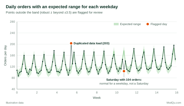
Figure 1 shows 16 weeks of hypothetical daily orders. The expected value for each day is the median for that weekday, adjusted for a gentle upward trend, and the robust standard deviation of the residuals is about 3.9 orders. Two days stand out. A Thursday with 203 orders, caused by a data load that duplicated part of the day's records, has a robust z-score of about 24. A Saturday with 104 orders, when a website outage lasted most of the afternoon, has a robust z-score of about −19.
A three-standard-deviation rule on the raw data finds neither. The duplicated Thursday has an ordinary z-score of 2.96, because the weekly cycle inflates the standard deviation, and the low Saturday sits close to the overall mean of about 125 orders. Only by modelling what each day should look like do both anomalies become obvious.
Detecting shifts, not just spikes
Some of the most important anomalies are not single points but sustained shifts: conversion rates that drift down after a website change, or a supplier whose defect rate creeps up. Statistical process control methods are designed for this. The cumulative sum (CUSUM) chart accumulates small deviations from a target and signals when their total becomes large (Page, 1954), and the exponentially weighted moving average chart gives more weight to recent observations (Roberts, 1959). Both detect small persistent changes much sooner than rules that look at one value at a time.
Multivariate anomalies
An observation can be normal on every single variable and still be anomalous in combination. An expense claim of $900 is unremarkable, and so is a one-night trip; a $900 claim for a one-night trip in a low-cost city is not. The Mahalanobis distance measures how far an observation lies from the centre of the data, taking account of the correlations between variables. Like the standard deviation, it suffers from masking when the mean and covariance are estimated from contaminated data. Rousseeuw and van Zomeren (1990) showed how robust estimates of location and scatter unmask such outliers, and the fast minimum covariance determinant algorithm made these estimates practical for large datasets (Rousseeuw & Van Driessen, 1999).
Machine learning methods
With many variables, or relationships that are far from linear, machine learning methods are often used:
- Isolation forest builds many random trees that split the data at random values. Anomalies, being few and different, are isolated in fewer splits than normal points, so the average path length gives an anomaly score (Liu et al., 2008). It is fast and scales well to large datasets.
- Local outlier factor compares the density around each point with the density around its neighbours, so it can find points that are unusual for their local region even when the data contain clusters of different density (Breunig et al., 2000).
Goldstein and Uchida (2016) compared many unsupervised anomaly detection algorithms on a range of benchmark datasets and found that performance varied considerably between datasets, with no single algorithm best overall. In practice it is sensible to compare two or three methods and to examine cases that all of them flag.
Fraud: when anomalies fight back
Fraud detection is the most demanding application. Bolton and Hand (2002) note that fraud is rare, that labelled examples are scarce and often delayed, and that fraudsters change their behaviour in response to detection. Supervised models trained on past fraud can only recognise patterns already seen, so unsupervised anomaly detection is used alongside them to catch new schemes. Its output is a ranked list for investigators, not a verdict.
Rarity also makes accuracy figures misleading. Suppose, hypothetically, that 1 in 1,000 transactions is fraudulent and a detector flags 99% of frauds while wrongly flagging only 1% of legitimate transactions. Among 100,000 transactions it would flag 99 frauds and 999 legitimate ones, so only about 9% of alerts would be fraud. Detectors for rare events should therefore be judged by the precision of their alerts and the share of true anomalies they find, not by overall accuracy, and alert volumes should be planned around the capacity of the people who must investigate them.
Practical guidance
- Define the purpose first. Cleaning data, detecting fraud and monitoring operations need different methods, thresholds and follow-up processes.
- Model context. Remove seasonal, weekly and trend patterns before looking for anomalies, and compare like with like, such as a store with similar stores.
- Use robust statistics. Estimate centres and spreads with medians, MAD or robust covariance so that anomalies do not hide each other.
- Manage the false alarm rate. Monitoring thousands of series every day guarantees many chance flags. Set thresholds with the volume of alerts in mind, or use procedures that control the false discovery rate (Benjamini & Hochberg, 1995).
- Investigate before acting. Check each flagged value against source records. Correct confirmed errors, keep genuine extremes and record what was done.
- Feed back the results. Investigators' conclusions provide labels that can be used to tune thresholds and to train supervised models later.
- In survey data, combine statistical flags for unusual answer patterns, such as implausibly fast completion or identical grid answers, with substantive checks before removing any respondent.
Common mistakes
- Deleting anomalies automatically. Extreme values are often real. Removing them can hide exactly the events the business needs to know about and can bias averages downwards.
- Using the mean and standard deviation to define unusual. Masking can make serious errors invisible.
- Ignoring seasonality and context. A rule applied to raw data flags normal peaks and misses abnormal troughs.
- Treating a flag as proof. An anomaly score indicates where to look, not what happened.
- Never revisiting the model. Business patterns change. A baseline from last year will flag this year's normal growth as anomalous.
Key takeaways
Anomaly detection finds the observations that do not fit, whether they are errors to be corrected or signals to be acted on. Use robust statistics rather than the mean and standard deviation, model the expected pattern before looking for departures from it, use control charts for gradual shifts and multivariate or machine learning methods when anomalies appear only in combination. Above all, treat flags as questions for people with business knowledge to answer, and manage the false alarm rate so that the real signals are not lost among false ones.
References
Benjamini, Y., & Hochberg, Y. (1995). Controlling the false discovery rate: A practical and powerful approach to multiple testing. Journal of the Royal Statistical Society Series B: Statistical Methodology, 57(1), 289–300. https://doi.org/10.1111/j.2517-6161.1995.tb02031.x
Bolton, R. J., & Hand, D. J. (2002). Statistical fraud detection: A review. Statistical Science, 17(3), 235–255. https://doi.org/10.1214/ss/1042727940
Breunig, M. M., Kriegel, H.-P., Ng, R. T., & Sander, J. (2000). LOF: Identifying density-based local outliers. ACM SIGMOD Record, 29(2), 93–104. https://doi.org/10.1145/335191.335388
Chandola, V., Banerjee, A., & Kumar, V. (2009). Anomaly detection. ACM Computing Surveys, 41(3), 1–58. https://doi.org/10.1145/1541880.1541882
Cleveland, R. B., Cleveland, W. S., McRae, J. E., & Terpenning, I. (1990). STL: A seasonal-trend decomposition procedure based on loess. Journal of Official Statistics, 6(1), 3–73.
Goldstein, M., & Uchida, S. (2016). A comparative evaluation of unsupervised anomaly detection algorithms for multivariate data. PLOS ONE, 11(4), Article e0152173. https://doi.org/10.1371/journal.pone.0152173
Hawkins, D. M. (1980). Identification of outliers. Springer. https://doi.org/10.1007/978-94-015-3994-4
Hoaglin, D. C., Iglewicz, B., & Tukey, J. W. (1986). Performance of some resistant rules for outlier labeling. Journal of the American Statistical Association, 81(396), 991–999. https://doi.org/10.1080/01621459.1986.10478363
Hubert, M., & Vandervieren, E. (2008). An adjusted boxplot for skewed distributions. Computational Statistics & Data Analysis, 52(12), 5186–5201. https://doi.org/10.1016/j.csda.2007.11.008
Hyndman, R. J., & Athanasopoulos, G. (2021). Forecasting: Principles and practice (3rd ed.). OTexts.
Leys, C., Ley, C., Klein, O., Bernard, P., & Licata, L. (2013). Detecting outliers: Do not use standard deviation around the mean, use absolute deviation around the median. Journal of Experimental Social Psychology, 49(4), 764–766. https://doi.org/10.1016/j.jesp.2013.03.013
Liu, F. T., Ting, K. M., & Zhou, Z.-H. (2008). Isolation forest. In 2008 Eighth IEEE International Conference on Data Mining (pp. 413–422). IEEE. https://doi.org/10.1109/ICDM.2008.17
Page, E. S. (1954). Continuous inspection schemes. Biometrika, 41(1–2), 100–115. https://doi.org/10.1093/biomet/41.1-2.100
Roberts, S. W. (1959). Control chart tests based on geometric moving averages. Technometrics, 1(3), 239–250. https://doi.org/10.1080/00401706.1959.10489860
Rousseeuw, P. J., & Hubert, M. (2011). Robust statistics for outlier detection. WIREs Data Mining and Knowledge Discovery, 1(1), 73–79. https://doi.org/10.1002/widm.2
Rousseeuw, P. J., & Van Driessen, K. (1999). A fast algorithm for the minimum covariance determinant estimator. Technometrics, 41(3), 212–223. https://doi.org/10.1080/00401706.1999.10485670
Rousseeuw, P. J., & van Zomeren, B. C. (1990). Unmasking multivariate outliers and leverage points. Journal of the American Statistical Association, 85(411), 633–639. https://doi.org/10.1080/01621459.1990.10474920
Tukey, J. W. (1977). Exploratory data analysis. Addison-Wesley.