
Statistics · Data science and machine learning
Conformal Prediction for Distribution-Free Uncertainty Knowledge
How conformal prediction wraps any predictive model in intervals with a guaranteed coverage rate, without distributional assumptions, and what that guarantee does and does not promise.
Machine learning models give point predictions: this customer will spend $84 next month, this respondent will rate the product 7 out of 10. Decisions need to know how far off such predictions can be. Classical prediction intervals rely on model assumptions such as normal errors, and many machine learning methods offer no intervals at all. Conformal prediction fills the gap. It turns the output of any model into prediction intervals (or, for classification, sets of plausible labels) that contain the true value with a chosen probability, such as 90%, using only the assumption that the data are exchangeable (Vovk et al., 2005; Shafer & Vovk, 2008).
Split conformal prediction
The simplest and most widely used version is split conformal prediction, also called inductive conformal prediction (Papadopoulos et al., 2002; Lei et al., 2018). It has four steps.
- Split the available data into a training set and a calibration set.
- Fit any model to the training set: a linear regression, a random forest or a neural network.
- For each of the n calibration cases, compute a nonconformity score, typically the absolute error |yi − ŷi|.
- For coverage 1 − α, take q̂ as the ⌈(n + 1)(1 − α)⌉-th smallest score. The interval for a new case is ŷ ± q̂.
The key result is that, if the calibration cases and the new case are exchangeable (for example, independent draws from the same population), the probability that the new value falls inside the interval is at least 1 − α. With continuous scores, it is also no more than 1 − α + 1 ÷ (n + 1), so the intervals are not needlessly wide (Lei et al., 2018). The intuition is simple. If the new case is exchangeable with the calibration cases, its score is equally likely to take any rank among the n + 1 scores, so it falls at or below the chosen rank with probability of at least 1 − α. No model for the errors is needed, only this symmetry. The guarantee holds in finite samples, whatever the model and whatever the shape of the error distribution. A poor model gives wide intervals, not invalid ones.
A worked example
Suppose a retailer predicts each customer's monthly spend with a gradient-boosted model and holds back 200 customers for calibration. Their absolute errors are skewed, with a long right tail. For 90% coverage, ⌈201 × 0.9⌉ = 181, so q̂ is the 181st smallest error, which in this hypothetical sample is $30.40.
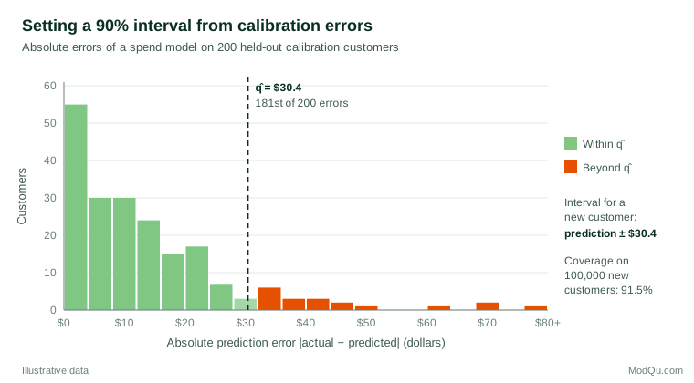
A customer predicted to spend $84 receives the interval $53.60 to $114.40. In a simulated check on 100,000 new customers, 91.5% of actual values fell inside their intervals. Coverage varies slightly from one calibration sample to another, but on average it is at least the promised 90%.
Making intervals adaptive
Intervals of the form ŷ ± q̂ have the same width for every customer, even though spend is far easier to predict for some than for others. Two refinements address this. Scores can be scaled by an estimate of each case's difficulty, or the method can be applied to quantile regression models. Conformalized quantile regression fits models for the lower and upper quantiles and then uses calibration scores to widen or narrow the band, giving intervals that are wider where the outcome is more variable while keeping the coverage guarantee (Romano et al., 2019).
Splitting sacrifices data. The jackknife+ uses leave-one-out fits so that every case contributes to both training and calibration, with a slightly weaker guarantee of at least 1 − 2α coverage (Barber et al., 2021).
What the guarantee does not cover
- Marginal, not conditional, coverage. The 90% holds on average over all customers. It can be 98% for typical customers and 70% for a rare segment. Check coverage by segment.
- Exchangeability. If the population changes between calibration and use, after a price change or in a new region, the guarantee can fail. Weighted methods offer some protection, with coverage loss bounded by how far the distribution has shifted (Barber et al., 2023), but recalibrating on recent data remains the safest course.
- No fix for bias. Conformal prediction measures the error a model actually makes. It does not correct survey nonresponse or a sample that differs systematically from the target population.
Practical guidance
- Use at least a few hundred calibration cases so q̂ is stable. With only 20 cases, a 95% interval is simply the largest error seen, which can swing widely between samples.
- Keep calibration data separate from all model tuning.
- For classification, conformal prediction produces sets of labels. A respondent's predicted segment might be {B} for a clear case and {A, B, C} for an ambiguous one; a large set signals a hard case worth human review (Angelopoulos & Bates, 2023).
- Report the coverage level and the calibration period alongside the intervals.
Key takeaways
Conformal prediction is a simple, assumption-light way to attach honest uncertainty to any predictive model. Its guarantee is finite-sample and distribution-free, but it is marginal and depends on exchangeability. Adaptive variants make intervals more informative, and regular recalibration keeps them valid as markets change (Angelopoulos & Bates, 2023).
References
Angelopoulos, A. N., & Bates, S. (2023). Conformal prediction: A gentle introduction. Foundations and Trends in Machine Learning, 16(4), 494–591. https://doi.org/10.1561/2200000101
Barber, R. F., Candès, E. J., Ramdas, A., & Tibshirani, R. J. (2021). Predictive inference with the jackknife+. The Annals of Statistics, 49(1), 486–507. https://doi.org/10.1214/20-AOS1965
Barber, R. F., Candès, E. J., Ramdas, A., & Tibshirani, R. J. (2023). Conformal prediction beyond exchangeability. The Annals of Statistics, 51(2), 816–845. https://doi.org/10.1214/23-AOS2276
Lei, J., G'Sell, M., Rinaldo, A., Tibshirani, R. J., & Wasserman, L. (2018). Distribution-free predictive inference for regression. Journal of the American Statistical Association, 113(523), 1094–1111. https://doi.org/10.1080/01621459.2017.1307116
Papadopoulos, H., Proedrou, K., Vovk, V., & Gammerman, A. (2002). Inductive confidence machines for regression. In T. Elomaa, H. Mannila, & H. Toivonen (Eds.), Machine learning: ECML 2002 (pp. 345–356). Springer. https://doi.org/10.1007/3-540-36755-1_29
Romano, Y., Patterson, E., & Candès, E. (2019). Conformalized quantile regression. In Advances in Neural Information Processing Systems (Vol. 32). Curran Associates.
Shafer, G., & Vovk, V. (2008). A tutorial on conformal prediction. Journal of Machine Learning Research, 9, 371–421.
Vovk, V., Gammerman, A., & Shafer, G. (2005). Algorithmic learning in a random world. Springer. https://doi.org/10.1007/b106715