
Statistics · Bayesian and computational
Ensemble Kalman Filters for Sequential Data Assimilation Knowledge
How the ensemble Kalman filter combines a model's forecast with each new batch of data to track quantities that cannot be observed directly, from weather to market indicators, and what can go wrong.
Weather forecasts are among the most visible successes of applied statistics. Every few hours, forecasting centres combine millions of new measurements from satellites, weather balloons and ground stations with the forecast from a physical model of the atmosphere, and produce a new best estimate of the current state of the weather. That estimate then becomes the starting point for the next forecast. The process of combining a model with incoming data in this way is called data assimilation, and one of its most widely used tools is the ensemble Kalman filter (EnKF).
The EnKF is not only for meteorologists. Any problem in which a quantity changes over time, cannot be measured directly and is observed only through noisy, incomplete data has the same structure: the true market share of a new product, the level of consumer confidence, the spread of an epidemic or the remaining capacity in a supply chain.
The sequential estimation problem
Data assimilation problems have two parts. A state describes the system at each time point, such as temperatures and winds across a grid, or the share of households that have adopted a product. A forecast model describes how the state moves from one time point to the next. Separately, observations are linked to the state through an observation model that allows for measurement error. A survey that estimates adoption from a sample of 500 households is such an observation: it is related to the true adoption share but differs from it by sampling error.
The goal is to estimate the state at each time, with an honest statement of uncertainty, as each new observation arrives. This is called filtering, and it is a Bayesian problem: the forecast acts as a prior, the new observation provides a likelihood, and the result, called the analysis, is the posterior. The analysis is then carried forward by the model to become the next prior. The cycle of forecast and update repeats indefinitely, so knowledge accumulates over time (Reich & Cotter, 2015).
The Kalman filter
For linear models with normally distributed errors, the exact solution was found by Kalman (1960). The Kalman filter keeps track of two things: the mean of the state and its covariance matrix, which records the uncertainty in each part of the state and how the uncertainties are related. At each update, the new estimate is a weighted average of the forecast and the observation. The weight, called the Kalman gain, depends on their relative uncertainty: a precise observation pulls the estimate strongly towards it, a noisy one only slightly. The Kalman filter remains the basis of state space methods in time series analysis, used for tasks such as estimating trends and seasonal patterns (Durbin & Koopman, 2012).
Two obstacles prevent the classical Kalman filter from being used directly in large applications. First, real forecast models are usually nonlinear, and the extended Kalman filter, which linearises them, can behave poorly. Second, the covariance matrix is enormous. A weather model may have a hundred million state variables, which means a covariance matrix with around 1016 elements, far too large to store or update.
The ensemble idea
Evensen (1994) proposed a practical way around both obstacles. Instead of storing the covariance matrix, the EnKF represents uncertainty with an ensemble: a collection of perhaps 20 to 100 possible states, each a plausible version of reality. The spread of the ensemble is the uncertainty, and the covariance matrix needed for the update is estimated from the ensemble members whenever it is needed, without ever being stored in full.
Each cycle has two steps:
- Forecast. Every ensemble member is run forward through the full nonlinear model, with random disturbances added to represent model error. Because members start from slightly different states, the ensemble spreads out where the system is unpredictable and stays tight where it is predictable.
- Analysis. When observations arrive, each member is moved towards the data using a Kalman gain computed from the ensemble's own covariance. Members that already agree with the data move little; those that disagree move more. The updated ensemble has a new mean and a smaller spread.
The method is a Monte Carlo approach in the forecast step and a linear, Kalman-type update in the analysis step. Houtekamer and Mitchell (1998) developed an EnKF for atmospheric data assimilation in the same period, and Evensen (2009) gives a full account of the theory and practice. Katzfuss et al. (2016) present the method in statistical language and show its relationship to standard Bayesian updating.
The update step in pictures
The most important feature of the EnKF is that observing one variable also updates others. Figure 1 shows a single update for a simple marketing example with two state variables: brand awareness, which a survey measures, and purchase intent, which it does not. The forecast ensemble shows a positive correlation between the two: members with higher awareness also tend to have higher intent.
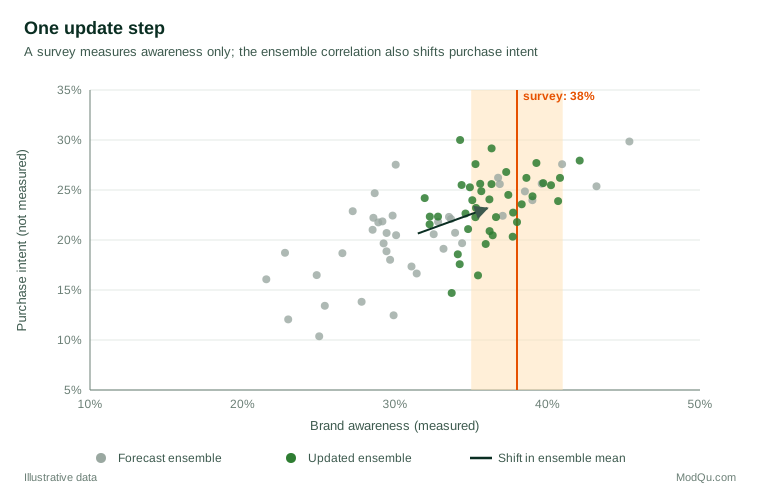
A survey then finds awareness of 38%, higher than the forecast of about 31%. The update moves the ensemble towards the survey value, to about 36%, not all the way, because the survey also has sampling error. It also moves purchase intent from about 21% to 23%, even though intent was never measured, because the ensemble covariance says that higher awareness usually comes with higher intent.
Variants of the filter
A difficulty emerged early. If every member is pulled towards exactly the same observation, the updated ensemble ends up with too little spread. Burgers et al. (1998) showed that adding random noise to the observations, giving each member its own perturbed copy, corrects this, and the resulting method is often called the stochastic or perturbed-observation EnKF.
The random perturbations introduce extra sampling noise, particularly with small ensembles. Ensemble square root filters avoid it by updating the ensemble mean and then transforming the deviations from the mean deterministically so that the spread has exactly the right size (Tippett et al., 2003). Examples include the ensemble adjustment Kalman filter (Anderson, 2001), the ensemble transform Kalman filter (Bishop et al., 2001) and the serial square root filter of Whitaker and Hamill (2002). The local ensemble transform Kalman filter (Hunt et al., 2007) performs the update independently in many small regions, which makes it very efficient on parallel computers and has led to its adoption by several operational weather centres.
Tuning: inflation and localisation
With a few dozen members standing in for a system with millions of variables, the ensemble estimate of the covariance is noisy and incomplete. Two practical remedies have become standard.
Covariance inflation counters the tendency of the ensemble to become overconfident. Sampling error, model error that is not represented and repeated updates all shrink the spread over time; if the ensemble becomes too tight, the filter gives new observations too little weight and drifts away from reality, a failure known as filter divergence. Inflation simply increases the spread of the forecast ensemble by a small factor, such as 1.05, before each update (Anderson & Anderson, 1999). Anderson (2007) showed how the inflation factor can itself be estimated as the filter runs.
Localisation deals with spurious correlations. With 40 members, the sample correlation between two unrelated variables will often be about 0.15 by chance, and the filter would act on it, letting an observation in one place alter estimates far away. Localisation multiplies the ensemble covariances by a function that falls to zero with distance, so that observations update only nearby variables (Hamill et al., 2001; Houtekamer & Mitchell, 1998). A compactly supported correlation function proposed by Gaspari and Cohn (1999) is widely used for this purpose. In non-spatial applications, such as a model of many market indicators, "distance" can be defined by how closely the variables are related in the model.
Tracking a quantity that cannot be observed directly
Figure 2 shows an EnKF tracking the share of households that have adopted a new product, using a simple growth model and weekly surveys with a sampling error of about 3.5 percentage points. The growth rate is not known in advance, so each ensemble member carries its own value of it, and the filter updates these values along with the adoption share. This technique, called state augmentation, allows the filter to learn model parameters from the data at the same time as it tracks the state.
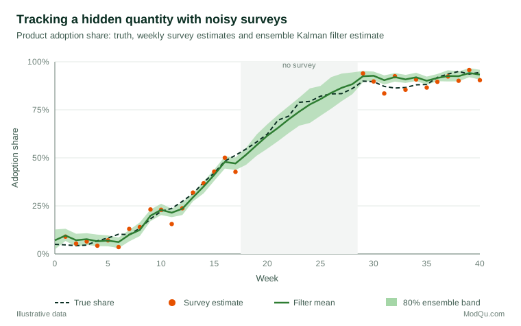
Three features stand out. First, the filter estimate is more accurate than the surveys themselves: in this simulation, the typical error of the filter mean is about 2.7 percentage points, against 3.7 for the individual surveys, because each estimate combines the latest survey with everything learned before. Second, during the 11 weeks without a survey, the filter continues to forecast using the model, and its uncertainty band widens to show that knowledge is getting older. Third, by week 40, the growth rate estimated by the ensemble has moved close to its true value, so the model's forecasts become more reliable as data accumulate.
Applications beyond the weather
Since its introduction, the EnKF has been used in oceanography, hydrology, petroleum reservoir modelling, ecology and epidemiology. Houtekamer and Zhang (2016) review its operational use in atmospheric prediction. In epidemiology, Shaman and Karspeck (2012) combined an EnKF with a disease transmission model and weekly estimates of influenza-like illness to forecast the timing of seasonal influenza peaks in United States cities several weeks ahead, an approach later used in real-time forecasting.
In business and social research, the same ideas apply wherever a model of change can be combined with noisy measurements: nowcasting economic indicators, tracking brand health from rolling surveys, updating demand estimates from daily sales or monitoring a customer base whose true size is only partly observed.
Limitations
The EnKF is fast and robust, but it is an approximation. Its update step assumes, in effect, that forecast uncertainty is roughly normal and that the relationship between state and observations is close to linear. When the forecast distribution has several peaks, for example when a system could be in one of two quite different regimes, the EnKF will average across them rather than choosing between them, and the result can be misleading.
Particle filters, which weight and resample ensemble members according to how well they match the data, make no such assumption (Gordon et al., 1993). However, Snyder et al. (2008) showed that the number of members a particle filter needs grows very quickly with the size of the problem, so that for high-dimensional systems particle filters collapse, with almost all the weight falling on a single member. The EnKF avoids this collapse precisely because of its linear update, which is why it, rather than the particle filter, dominates large-scale applications.
Other limitations follow from the tuning. Inflation and localisation settings are often chosen by trial and error, and poorly chosen values can lead to an overconfident or unstable filter. The method also depends on the quality of the forecast model: a model with systematic errors will pull the estimates away from the truth between observations, and the ensemble spread will not show it unless model error is represented explicitly.
Practical guidance
- Start with a clear state and observation model. Write down what is being tracked, how it changes and how each data source relates to it, including its error.
- Check the ensemble spread. Over many cycles, the spread should match the actual differences between forecasts and observations. A spread that is consistently too small calls for more inflation.
- Use localisation with large state vectors. Without it, small ensembles will create false links between unrelated variables.
- Represent model error. Add random disturbances or use inflation to reflect the fact that the model is imperfect.
- Validate against held-out data. Hold back some observations and check whether the filter predicts them as well as its uncertainty bands claim.
Key takeaways
The ensemble Kalman filter turns a stream of incomplete, noisy observations into a continuously updated estimate of a hidden state, using a small ensemble of model runs to represent uncertainty. Its update step pulls each member towards the data and, through the ensemble's covariance, also revises quantities that were not measured. Inflation and localisation make it work with small ensembles in very large systems. It is an approximation that struggles with strongly non-normal uncertainty, but its speed and robustness have made it a standard tool in weather prediction and a useful one wherever knowledge about a changing system must be refreshed as each new piece of data arrives.
References
Anderson, J. L. (2001). An ensemble adjustment Kalman filter for data assimilation. Monthly Weather Review, 129(12), 2884–2903. https://doi.org/10.1175/1520-0493(2001)129<2884:AEAKFF>2.0.CO;2
Anderson, J. L. (2007). An adaptive covariance inflation error correction algorithm for ensemble filters. Tellus A: Dynamic Meteorology and Oceanography, 59(2), 210–224. https://doi.org/10.1111/j.1600-0870.2006.00216.x
Anderson, J. L., & Anderson, S. L. (1999). A Monte Carlo implementation of the nonlinear filtering problem to produce ensemble assimilations and forecasts. Monthly Weather Review, 127(12), 2741–2758. https://doi.org/10.1175/1520-0493(1999)127<2741:AMCIOT>2.0.CO;2
Bishop, C. H., Etherton, B. J., & Majumdar, S. J. (2001). Adaptive sampling with the ensemble transform Kalman filter. Part I: Theoretical aspects. Monthly Weather Review, 129(3), 420–436. https://doi.org/10.1175/1520-0493(2001)129<0420:ASWTET>2.0.CO;2
Burgers, G., van Leeuwen, P. J., & Evensen, G. (1998). Analysis scheme in the ensemble Kalman filter. Monthly Weather Review, 126(6), 1719–1724. https://doi.org/10.1175/1520-0493(1998)126<1719:ASITEK>2.0.CO;2
Durbin, J., & Koopman, S. J. (2012). Time series analysis by state space methods (2nd ed.). Oxford University Press. https://doi.org/10.1093/acprof:oso/9780199641178.001.0001
Evensen, G. (1994). Sequential data assimilation with a nonlinear quasi-geostrophic model using Monte Carlo methods to forecast error statistics. Journal of Geophysical Research: Oceans, 99(C5), 10143–10162. https://doi.org/10.1029/94JC00572
Evensen, G. (2009). Data assimilation: The ensemble Kalman filter (2nd ed.). Springer. https://doi.org/10.1007/978-3-642-03711-5
Gaspari, G., & Cohn, S. E. (1999). Construction of correlation functions in two and three dimensions. Quarterly Journal of the Royal Meteorological Society, 125(554), 723–757. https://doi.org/10.1002/qj.49712555417
Gordon, N. J., Salmond, D. J., & Smith, A. F. M. (1993). Novel approach to nonlinear/non-Gaussian Bayesian state estimation. IEE Proceedings F: Radar and Signal Processing, 140(2), 107–113. https://doi.org/10.1049/ip-f-2.1993.0015
Hamill, T. M., Whitaker, J. S., & Snyder, C. (2001). Distance-dependent filtering of background error covariance estimates in an ensemble Kalman filter. Monthly Weather Review, 129(11), 2776–2790. https://doi.org/10.1175/1520-0493(2001)129<2776:DDFOBE>2.0.CO;2
Houtekamer, P. L., & Mitchell, H. L. (1998). Data assimilation using an ensemble Kalman filter technique. Monthly Weather Review, 126(3), 796–811. https://doi.org/10.1175/1520-0493(1998)126<0796:DAUAEK>2.0.CO;2
Houtekamer, P. L., & Zhang, F. (2016). Review of the ensemble Kalman filter for atmospheric data assimilation. Monthly Weather Review, 144(12), 4489–4532. https://doi.org/10.1175/MWR-D-15-0440.1
Hunt, B. R., Kostelich, E. J., & Szunyogh, I. (2007). Efficient data assimilation for spatiotemporal chaos: A local ensemble transform Kalman filter. Physica D: Nonlinear Phenomena, 230(1–2), 112–126. https://doi.org/10.1016/j.physd.2006.11.008
Kalman, R. E. (1960). A new approach to linear filtering and prediction problems. Journal of Basic Engineering, 82(1), 35–45. https://doi.org/10.1115/1.3662552
Katzfuss, M., Stroud, J. R., & Wikle, C. K. (2016). Understanding the ensemble Kalman filter. The American Statistician, 70(4), 350–357. https://doi.org/10.1080/00031305.2016.1141709
Reich, S., & Cotter, C. (2015). Probabilistic forecasting and Bayesian data assimilation. Cambridge University Press. https://doi.org/10.1017/CBO9781107706804
Shaman, J., & Karspeck, A. (2012). Forecasting seasonal outbreaks of influenza. Proceedings of the National Academy of Sciences, 109(50), 20425–20430. https://doi.org/10.1073/pnas.1208772109
Snyder, C., Bengtsson, T., Bickel, P., & Anderson, J. (2008). Obstacles to high-dimensional particle filtering. Monthly Weather Review, 136(12), 4629–4640. https://doi.org/10.1175/2008MWR2529.1
Tippett, M. K., Anderson, J. L., Bishop, C. H., Hamill, T. M., & Whitaker, J. S. (2003). Ensemble square root filters. Monthly Weather Review, 131(7), 1485–1490. https://doi.org/10.1175/1520-0493(2003)131<1485:ESRF>2.0.CO;2
Whitaker, J. S., & Hamill, T. M. (2002). Ensemble data assimilation without perturbed observations. Monthly Weather Review, 130(7), 1913–1924. https://doi.org/10.1175/1520-0493(2002)130<1913:EDAWPO>2.0.CO;2