
Statistics · Tests and models
Dynamic Factor Models for High-Dimensional Time-Series Knowledge
How dynamic factor models summarise dozens or hundreds of related time series with a few common factors, and how they support nowcasting, composite indices and tracking studies.
Organisations rarely watch a single number. An economist follows hundreds of monthly indicators of output, prices, employment and sentiment. A brand team tracks awareness, consideration, satisfaction and purchase intent across many markets, waves and segments. A retailer monitors sales across thousands of products and stores. Each series is noisy, many are released at different times, and some have gaps. Yet the series often move together, because they respond to a small number of underlying forces: the business cycle, the strength of a brand, the general mood of consumers.
Dynamic factor models (DFMs) turn that observation into a statistical tool. They assume that a large panel of time series is driven by a few unobserved common factors that evolve over time, plus series-specific noise. Estimating the factors compresses hundreds of indicators into a handful of interpretable signals, and the model can then be used to forecast, to build composite indices, to fill in missing observations and to read the current state of a system before official figures arrive. This article explains how DFMs work, how they are estimated, and where they help, and mislead, in business and survey research.
The idea: many series, few drivers
Suppose there are N time series observed over T periods. In a DFM, each series xit is written as a weighted combination of r common factors plus an idiosyncratic component:
xit = λi1f1t + λi2f2t + … + λirfrt + eit
The factors ft are shared by all series, the loadings λi describe how strongly each series responds to each factor, and eit captures everything specific to series i, including measurement error. The "dynamic" part is a second equation describing how the factors themselves evolve, usually as a vector autoregression:
ft = A1ft−1 + … + Apft−p + ut
The first equation is a measurement equation and the second a transition equation, so a DFM is a state space model of the kind introduced by Kalman (1960) and developed for statistics and econometrics by Durbin and Koopman (2012). The key feature is that r is small, often between one and eight, even when N runs into the hundreds. The model therefore replaces an unmanageable number of cross-correlations with a compact description of co-movement.
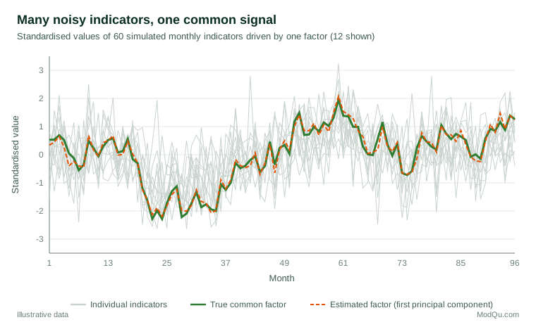
Figure 1 shows the idea with simulated data. Sixty monthly indicators are generated from one slowly moving factor plus independent noise. Individually, each series looks erratic. Averaged across the panel in the right way, the noise cancels and the common factor emerges clearly.
From classical factor analysis to large panels
Factor analysis has a long history in psychology, where it was used to explain correlations between test scores with a few latent abilities. Applying the idea to economic time series began in the 1970s, when researchers showed that a few dynamic factors could account for much of the co-movement among macroeconomic variables (Stock & Watson, 2016). Those early models were estimated by maximum likelihood with a small number of series.
A first breakthrough was the composite index. Stock and Watson (1989) built a coincident index of the United States economy as the single common factor of four monthly indicators, estimated with the Kalman filter, giving a statistical foundation to the business cycle indices long produced by hand. Mariano and Murasawa (2003) extended the approach to combine monthly and quarterly series, and Aruoba et al. (2009) built a daily index of business conditions from indicators observed at very different frequencies.
The second breakthrough was the realisation that having many series is a strength rather than a burden. Chamberlain and Rothschild (1983) introduced the approximate factor structure, in which idiosyncratic components may be weakly correlated with one another, a more realistic assumption for large panels. Building on this, Stock and Watson (2002a, 2002b) showed that the factors can be estimated consistently by principal components when both N and T are large, and that forecasts built on a few such "diffusion indexes" outperformed standard benchmarks for many United States macroeconomic series. Bai (2003) provided the asymptotic theory for the estimated factors and loadings, including standard errors. At around the same time, Forni et al. (2000, 2005) developed the generalised dynamic factor model, which estimates factors in the frequency domain and allows richer lag structures.
How the models are estimated
Principal components
The simplest method standardises each series and takes the first r principal components of the panel as the factor estimates. It is fast, needs no distributional assumptions and works well when the panel is large and balanced. Principal components estimate the space spanned by the factors rather than each factor's precise meaning, so individual factors are identified only up to a rotation. For forecasting this rarely matters; for interpretation it does, and analysts often rotate or label factors by looking at which series load most heavily on them.
State space and the Kalman filter
Writing the model in state space form allows estimation by maximum likelihood, with the Kalman filter computing the likelihood and the Kalman smoother producing the best estimate of the factors given all the data. The state space approach handles missing observations, mixed frequencies and series that start or end at different dates in a natural way, because the filter simply skips the update step when a value is absent. Shumway and Stoffer (1982) showed how to combine the Kalman smoother with the expectation-maximisation (EM) algorithm of Dempster et al. (1977) to estimate state space models, and this combination remains the standard route (Shumway & Stoffer, 2017).
For a long time maximum likelihood was considered impractical for large panels. Doz et al. (2011) proposed a two-step estimator: obtain initial factors by principal components, estimate the model parameters from them, then re-estimate the factors with the Kalman smoother. Doz et al. (2012) showed that full quasi-maximum likelihood via EM is also feasible and consistent for large approximate factor models, even when the idiosyncratic structure is misspecified. Bańbura and Modugno (2014) extended the EM algorithm to data sets with an arbitrary pattern of missing values, which is exactly the situation of real-time data.
Bayesian estimation
Bayesian versions treat factors and parameters as unknowns to be sampled by Markov chain Monte Carlo. They are convenient when prior information is available, for instance on which series should load on which factor, and when full uncertainty about the factors is needed. They are slower than principal components but scale well with modern software.
Comparing the main approaches
| Approach | Strengths | Weaknesses | Typical use |
|---|---|---|---|
| Principal components | Fast, simple, no distributional assumptions, consistent for large N and T | Needs a balanced panel; no direct handling of missing values or mixed frequencies | Forecasting with diffusion indexes, first exploration |
| State space with Kalman filter (maximum likelihood or EM) | Handles missing data, ragged edges and mixed frequencies; gives smoothed factors with uncertainty | More assumptions and more computation; sensitive to starting values | Nowcasting, composite indices, real-time monitoring |
| Generalised dynamic factor model | Rich lag structure, estimated in the frequency domain | More complex to implement and explain | Research on macroeconomic co-movement |
| Bayesian | Uses prior information, full posterior uncertainty | Slower; results depend on priors | Structured models with known blocks of series |
The choice is less important than it seems for well-behaved, large panels, because the different estimators tend to produce very similar factors. It matters more when panels are short, unbalanced or released at different times, which is where state space methods earn their extra complexity (Doz et al., 2011).
Choosing the number of factors
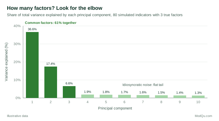
The number of factors r is the main modelling choice. Too few and real common movements are pushed into the noise; too many and the model starts fitting idiosyncratic quirks. A scree plot, showing the share of variance explained by each principal component, is the usual first look (Figure 2). With three true factors and moderate noise, the first three components stand out, and the remainder form a flat tail.
Real data are rarely so tidy. Bai and Ng (2002) proposed information criteria that penalise additional factors in a way that depends on both N and T, and these criteria are widely used for static factors. Hallin and Liška (2007) developed a corresponding criterion for the generalised dynamic factor model. In practice, analysts combine formal criteria with judgement about interpretability and with out-of-sample forecasting performance, and check that conclusions do not change much if one factor is added or removed.
What dynamic factor models are used for
Nowcasting
Official statistics such as gross domestic product are published with a delay of weeks or months, while many related indicators, including surveys, financial prices and administrative data, arrive much sooner. Nowcasting uses those early indicators to estimate the current quarter before the official number is released. Giannone et al. (2008) built a DFM that updates its estimate every time a new data release arrives, and showed that the precision of the nowcast improves steadily through the quarter as information accumulates. Their framework, which handles the "ragged edge" of data sets in which recent values are missing for slow-release series, is now used by many central banks. Survey indicators, such as business and consumer confidence, often carry much of the weight early in the quarter because they are available first.
Forecasting
Factor-augmented forecasts add a few estimated factors to a simple forecasting regression. Because the factors summarise information from many series, they can improve forecasts without the overfitting that would result from including all the series directly (Stock & Watson, 2002b). Boivin and Ng (2006) cautioned that more data are not always better: adding series that are noisy or dominated by a factor irrelevant to the target can make the estimated factors less useful for forecasting, so the composition of the panel matters.
Structural analysis
Bernanke et al. (2005) combined factors with a vector autoregression in the factor-augmented VAR (FAVAR), to study how monetary policy affects a wide range of economic variables at once. The same idea appears in business settings when analysts want to trace how a shock to one driver, such as a price change or a marketing campaign, spreads through many related indicators.
Composite indices and tracking studies
Beyond macroeconomics, DFMs offer a principled way to build composite indicators. A brand health index, a consumer sentiment index or a regional activity index can be defined as the common factor of the relevant series, with weights estimated from the data rather than chosen arbitrarily, and with a measure of uncertainty attached. For continuous survey trackers, a DFM can smooth wave-to-wave sampling noise while preserving genuine turning points, because the factor borrows strength from all the questions that move with it.
A worked example: a consumer confidence factor
Consider a hypothetical monthly tracking survey with 24 questions about household finances, buying intentions, job security and expectations for the economy, each reported as a balance score for 18 regions. That is 432 monthly series. Many are noisy because regional samples are small.
- Prepare the data. Transform each series to be roughly stationary, for example by working with levels of balance scores that fluctuate around a stable mean, or month-on-month changes for trending series. Standardise each series so that no single question dominates because of its scale.
- Choose the number of factors. A scree plot and the Bai and Ng (2002) criteria suggest two factors. The first loads on almost every question and region and is interpreted as general consumer confidence; the second loads positively on questions about personal finances and negatively on questions about the national economy, capturing the gap between how people see their own situation and the country's.
- Estimate by state space. Fit the model with the EM algorithm and Kalman smoother, so that months with missing regional data and the latest month, where some regions are not yet complete, are handled without discarding information.
- Use the results. The smoothed first factor is published as a confidence index with an uncertainty band. Each regional series can be decomposed into the part explained by the common factors and the regional idiosyncratic component, which highlights regions moving against the national trend.
In this illustration the factor index is far smoother than any single regional series, and it signals turning points earlier than a simple average because it weights more informative questions more heavily.
Reading the output
Three outputs deserve attention. The loadings show how each series relates to each factor; a question with a large loading on the confidence factor is a good single proxy for it, while a question with a near-zero loading is mostly measuring something else. The communality of a series, the share of its variance explained by the common factors, shows how much of its movement is shared and how much is specific; in the example, national-level questions may have communalities above 0.8, while small regional series may sit below 0.3 because sampling noise dominates. Finally, the idiosyncratic components are themselves informative: a region whose idiosyncratic component drifts steadily upwards is diverging from the national pattern for reasons that deserve investigation, perhaps a local employer opening or a regional sample problem.
Because the estimated factor carries a standard error, a change in the index from one month to the next can be judged against its uncertainty rather than read as news every time it moves. This is one of the main advantages over a simple average of indicators, which offers no such measure.
Dynamic factor models in survey and market research
Although DFMs grew up in macroeconomics, the structure they assume is common in survey and business data.
- Brand and customer trackers. Continuous trackers ask many related questions every wave. A factor model can separate the shared movement in brand perceptions from item-specific noise, giving a more stable measure of brand health and showing which attributes move with it.
- Panels of markets or stores. Sales across many stores or regions often share national factors (season, promotions, the economy) and regional factors. Separating them helps identify where local performance genuinely differs.
- Combining survey and administrative data. Survey indicators are timely but noisy; administrative and transactional data are precise but slow or partial. A state space DFM can combine them, using each source for what it does best, much as Giannone et al. (2008) combine soft survey indicators with hard data.
- Small-sample smoothing. Where subgroup samples are small, the common factor lets each subgroup series borrow strength from the others, in a time-series counterpart to small area estimation.
In each case the same caution applies: a factor is a statistical summary of co-movement, and its business meaning has to be established from the loadings, from subject-matter knowledge and from how it behaves around known events.
Limitations and common mistakes
DFMs are powerful, but several pitfalls recur.
- Non-stationarity. Factor models assume the series fluctuate around stable means and variances. Trending series must be transformed first, or the leading factor will simply be a common trend that looks impressive but says little. Unit-root tests and careful differencing are part of the preparation (Stock & Watson, 2016).
- Structural breaks. Loadings may change when the economy, a market or a survey method changes. A break in questionnaire wording or mode can appear as a shift in the factor that has nothing to do with the underlying construct. Monitoring residuals and re-estimating over rolling windows helps.
- Over-interpreting factors. Factors are identified only up to rotation, and names such as "confidence" or "brand strength" are interpretations. Labels should be justified by the loadings and checked for stability over time.
- Panel composition. A panel dominated by one type of series, for example many closely related price indices, will produce a factor that mainly reflects that block. Balancing the panel or using a model with block-specific factors prevents this (Boivin & Ng, 2006).
- Ignoring uncertainty. Estimated factors are not observed data. With small N or short T they can be imprecise, and their standard errors should be reported (Bai, 2003).
- Evaluating on revised data. Nowcasting accuracy should be evaluated with the data as they were available at the time, not with later revised values, otherwise performance will be overstated (Giannone et al., 2008).
Practical guidance
- Start with principal components. They give a quick and robust first estimate and a scree plot. Move to a state space model when missing data, mixed frequencies or real-time updating matter.
- Select series with purpose. Include indicators that are timely, relevant to the target and not merely duplicates of one another.
- Test forecasting value out of sample. Compare factor-based forecasts with simple benchmarks on a hold-out period before relying on them (Stock & Watson, 2002a).
- Report the loadings. Show which series drive each factor, so that users can understand and challenge the index.
- Keep it reproducible. Document transformations, the number of factors and the estimation window, and archive the data vintages used. Surveys of methods and software (Bai & Ng, 2008; Stock & Watson, 2011) provide good checklists.
Key takeaways
Dynamic factor models exploit a simple regularity: when many series move together, a few common factors carry most of the information. Estimating those factors, by principal components or by state space methods with the Kalman filter, turns a large, noisy and incomplete panel into a small set of signals that can be tracked, forecast and explained. They underpin nowcasts of the economy, composite indices and smoother readings of continuous survey trackers. Used with care over stationarity, structural change, panel composition and uncertainty, they turn high-dimensional time series into clear and timely knowledge.
References
Aruoba, S. B., Diebold, F. X., & Scotti, C. (2009). Real-time measurement of business conditions. Journal of Business & Economic Statistics, 27(4), 417–427. https://doi.org/10.1198/jbes.2009.07205
Bai, J. (2003). Inferential theory for factor models of large dimensions. Econometrica, 71(1), 135–171. https://doi.org/10.1111/1468-0262.00392
Bai, J., & Ng, S. (2002). Determining the number of factors in approximate factor models. Econometrica, 70(1), 191–221. https://doi.org/10.1111/1468-0262.00273
Bai, J., & Ng, S. (2008). Large dimensional factor analysis. Foundations and Trends in Econometrics, 3(2), 89–163. https://doi.org/10.1561/0800000002
Bańbura, M., & Modugno, M. (2014). Maximum likelihood estimation of factor models on datasets with arbitrary pattern of missing data. Journal of Applied Econometrics, 29(1), 133–160. https://doi.org/10.1002/jae.2306
Bernanke, B. S., Boivin, J., & Eliasz, P. (2005). Measuring the effects of monetary policy: A factor-augmented vector autoregressive (FAVAR) approach. The Quarterly Journal of Economics, 120(1), 387–422. https://doi.org/10.1162/0033553053327452
Boivin, J., & Ng, S. (2006). Are more data always better for factor analysis? Journal of Econometrics, 132(1), 169–194. https://doi.org/10.1016/j.jeconom.2005.01.027
Chamberlain, G., & Rothschild, M. (1983). Arbitrage, factor structure, and mean-variance analysis on large asset markets. Econometrica, 51(5), 1281–1304. https://doi.org/10.2307/1912275
Dempster, A. P., Laird, N. M., & Rubin, D. B. (1977). Maximum likelihood from incomplete data via the EM algorithm. Journal of the Royal Statistical Society Series B: Statistical Methodology, 39(1), 1–22. https://doi.org/10.1111/j.2517-6161.1977.tb01600.x
Doz, C., Giannone, D., & Reichlin, L. (2011). A two-step estimator for large approximate dynamic factor models based on Kalman filtering. Journal of Econometrics, 164(1), 188–205. https://doi.org/10.1016/j.jeconom.2011.02.012
Doz, C., Giannone, D., & Reichlin, L. (2012). A quasi-maximum likelihood approach for large, approximate dynamic factor models. The Review of Economics and Statistics, 94(4), 1014–1024. https://doi.org/10.1162/REST_a_00225
Durbin, J., & Koopman, S. J. (2012). Time series analysis by state space methods (2nd ed.). Oxford University Press. https://doi.org/10.1093/acprof:oso/9780199641178.001.0001
Forni, M., Hallin, M., Lippi, M., & Reichlin, L. (2000). The generalized dynamic-factor model: Identification and estimation. The Review of Economics and Statistics, 82(4), 540–554. https://doi.org/10.1162/003465300559037
Forni, M., Hallin, M., Lippi, M., & Reichlin, L. (2005). The generalized dynamic factor model: One-sided estimation and forecasting. Journal of the American Statistical Association, 100(471), 830–840. https://doi.org/10.1198/016214504000002050
Giannone, D., Reichlin, L., & Small, D. (2008). Nowcasting: The real-time informational content of macroeconomic data. Journal of Monetary Economics, 55(4), 665–676. https://doi.org/10.1016/j.jmoneco.2008.05.010
Hallin, M., & Liška, R. (2007). Determining the number of factors in the general dynamic factor model. Journal of the American Statistical Association, 102(478), 603–617. https://doi.org/10.1198/016214506000001275
Kalman, R. E. (1960). A new approach to linear filtering and prediction problems. Journal of Basic Engineering, 82(1), 35–45. https://doi.org/10.1115/1.3662552
Mariano, R. S., & Murasawa, Y. (2003). A new coincident index of business cycles based on monthly and quarterly series. Journal of Applied Econometrics, 18(4), 427–443. https://doi.org/10.1002/jae.695
Shumway, R. H., & Stoffer, D. S. (1982). An approach to time series smoothing and forecasting using the EM algorithm. Journal of Time Series Analysis, 3(4), 253–264. https://doi.org/10.1111/j.1467-9892.1982.tb00349.x
Shumway, R. H., & Stoffer, D. S. (2017). Time series analysis and its applications: With R examples (4th ed.). Springer. https://doi.org/10.1007/978-3-319-52452-8
Stock, J. H., & Watson, M. W. (1989). New indexes of coincident and leading economic indicators. NBER Macroeconomics Annual, 4, 351–394. https://doi.org/10.1086/654119
Stock, J. H., & Watson, M. W. (2002a). Forecasting using principal components from a large number of predictors. Journal of the American Statistical Association, 97(460), 1167–1179. https://doi.org/10.1198/016214502388618960
Stock, J. H., & Watson, M. W. (2002b). Macroeconomic forecasting using diffusion indexes. Journal of Business & Economic Statistics, 20(2), 147–162. https://doi.org/10.1198/073500102317351921
Stock, J. H., & Watson, M. W. (2011). Dynamic factor models. In M. P. Clements & D. F. Hendry (Eds.), The Oxford handbook of economic forecasting (pp. 35–60). Oxford University Press. https://doi.org/10.1093/oxfordhb/9780195398649.013.0003
Stock, J. H., & Watson, M. W. (2016). Dynamic factor models, factor-augmented vector autoregressions, and structural vector autoregressions in macroeconomics. In J. B. Taylor & H. Uhlig (Eds.), Handbook of macroeconomics (Vol. 2, pp. 415–525). Elsevier. https://doi.org/10.1016/bs.hesmac.2016.04.002