
Statistics · Tests and models
Compositional Data Analysis for Proportional Knowledge Structures
Shares, budgets and mixes that sum to 100% carry only relative information. This article explains why standard statistics mislead with such data and how log-ratio methods analyse them properly.
A great deal of business data comes as parts of a whole. A household splits its budget between groceries, dining, entertainment and travel. A brand's sales come from stores, websites and marketplaces. A survey asks respondents to "allocate 100 points" across product features. Market shares, vote shares, channel mixes, time-use diaries and share-of-wallet measures all have the same structure: a set of non-negative parts that add up to a fixed total, usually 1 or 100%. Statisticians call these compositional data.
The fixed total seems harmless, but it changes the nature of the data. If one share rises, at least one other must fall, whatever is happening in the world. Standard tools such as correlations, means, standard deviations and linear regression on raw percentages ignore this constraint and can give misleading answers. Compositional data analysis, developed mainly by John Aitchison in the 1980s, offers a coherent alternative based on log-ratios between parts (Aitchison, 1982, 1986). This article explains the problem, the main log-ratio tools, how to apply them to survey and market data, and where their limits lie.
What makes data compositional
A composition is a vector of D positive parts x1, …, xD whose information lies in their relative sizes. Multiplying all parts by the same constant (reporting spending in pounds instead of percentages, say) should not change any conclusion. The operation that rescales a vector to a fixed total is called closure:
C(x) = (x1 ÷ Σxj, …, xD ÷ Σxj)
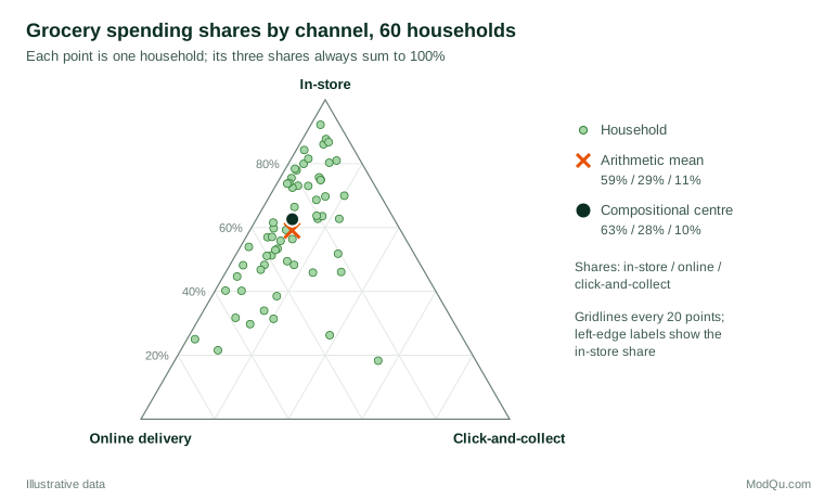
All closed compositions with D parts live in a restricted space called the simplex. For three parts, the simplex can be drawn as a triangle, the ternary diagram in Figure 2. Each corner represents 100% of one part, and every point inside the triangle is a possible mix.
Aitchison (1986) set out three principles that a sound analysis of compositions should respect. Scale invariance: results should not depend on the total. Permutation invariance: results should not depend on the order in which parts are listed. Subcompositional coherence: conclusions about a set of parts should not change when other parts are added or removed from the analysis. Standard methods applied to raw shares fail the third principle, as the next section shows. Later work built a full geometry for the simplex on these principles (Pawlowsky-Glahn et al., 2015).
A single proportion, such as the share of customers who renewed, is not a composition in this sense; logistic or beta regression usually suits it better.
Why standard methods mislead
Spurious correlation
The problem was first identified by Pearson (1897), who showed that ratios sharing a common denominator can be correlated even when the underlying quantities are independent. He called this spurious correlation. Chayes (1960) later showed that the constant sum forces a negative bias on correlations between parts: since each part's covariances with the others must sum to minus its own variance, at least one covariance in every row must be negative, whatever the true relationships.
Figure 1 illustrates the effect with 1,000 simulated households whose monthly spending on four categories is generated independently, so the true correlations between amounts are zero. Correlations between the raw amounts are close to zero, as they should be. Converted to shares of the four-part total, the correlations become slightly negative. Recalculated as shares of a three-part subcomposition that excludes travel, they become strongly negative: −0.77 for groceries and dining. The data have not changed; only the parts included have. A reported trade-off between grocery and dining shares would be an artefact of arithmetic.

The ratio between two parts, by contrast, is unaffected by closure. Dining divided by entertainment is the same whether computed from pounds, from four-part shares or from three-part shares. This is the key insight behind the log-ratio approach: ratios between parts carry the relative information that compositions contain, and they are subcompositionally coherent.
Means, spreads and predictions
Other standard summaries also behave poorly. Standard deviations of shares are hard to interpret because a part near 0% or 100% cannot vary much in absolute terms. Linear regression on raw shares can predict values below zero or above 100%, and the predicted parts need not sum to the total. Even single-part analyses are affected: Filzmoser et al. (2009) show that routine univariate statistics on closed environmental data, such as outlier rules and confidence limits, can be distorted and recommend log-ratio alternatives.
Relative change also matters. A share rising from 1% to 2% has doubled; one moving from 50% to 51% has barely changed. Both are one percentage point, but only log-ratios reflect the difference.
The log-ratio toolkit
Aitchison (1982, 1986) proposed moving compositions out of the simplex into ordinary real space by taking logarithms of ratios between parts. Standard multivariate methods can then be applied to the transformed values, and results can be transformed back to compositions. Three transformations are in common use.
Additive log-ratio (alr). Each part is divided by a chosen reference part, and the logarithm is taken, giving D − 1 values:
alr(x) = (ln(x1 ÷ xD), …, ln(xD−1 ÷ xD))
The alr is easy to explain and natural when one part is a meaningful baseline, such as in-store sales, but distances in alr space depend on the reference part chosen.
Centred log-ratio (clr). Each part is divided by the geometric mean g(x) of all parts:
clr(x) = (ln(x1 ÷ g(x)), …, ln(xD ÷ g(x)))
The clr treats all parts symmetrically and preserves distances, which makes it the usual basis for principal component analysis and biplots. Its values sum to zero, so the clr covariance matrix is singular and the transformed values cannot be used directly in some models.
Isometric log-ratio (ilr). Egozcue et al. (2003) introduced orthonormal coordinates for the simplex, giving D − 1 unconstrained values that preserve distances and angles. Any standard statistical method can be applied to ilr coordinates. A particularly interpretable form is the balance, built from a sequential binary partition of the parts (Egozcue & Pawlowsky-Glahn, 2005). A balance compares the geometric mean of one group of parts with that of another:
b = √(rs ÷ (r + s)) × ln(g(x+) ÷ g(x−))
where r and s are the numbers of parts in the two groups x+ and x−. With well-chosen partitions, balances answer business questions directly: "essentials versus discretionary spending" or "digital versus physical channels".
The natural measure of difference between two compositions is the Aitchison distance, the ordinary Euclidean distance between their clr vectors. It respects scale invariance and subcompositional dominance (distances in a subcomposition are never larger than in the full composition), properties that ordinary distances on percentages lack (Aitchison et al., 2000).
A worked example
A hypothetical household spends 40% of its discretionary budget on groceries, 20% on dining, 10% on entertainment and 30% on travel. The geometric mean of the four shares is 22.1, so the clr values are:
| Part | Share | clr value |
|---|---|---|
| Groceries | 40% | 0.59 |
| Dining | 20% | −0.10 |
| Entertainment | 10% | −0.80 |
| Travel | 30% | 0.30 |
Positive values mark parts above the household's "typical" part; negative values mark parts below it. A balance between food (groceries, dining) and leisure (entertainment, travel) uses r = s = 2, so the coefficient is 1 and the balance is ln(28.3 ÷ 17.3) = 0.49, food spending being about 1.6 times leisure spending in geometric-mean terms.
Suppose the household then moves 5 points from travel to dining (40%, 25%, 10%, 25%). The food–leisure balance rises to 0.69, meaning food spending is now twice leisure spending. The log-ratio of travel to entertainment falls from 1.10 to 0.92, while the log-ratio of groceries to entertainment is unchanged at 1.39. The log-ratio summary reports exactly which relative positions moved and which did not, something a list of percentage-point changes conveys only indirectly.
Describing a set of compositions
For a sample of compositions, the recommended measure of centre is the closed geometric mean: take the geometric mean of each part across observations, then close the result to 100%. It is the mean in clr space transformed back, and it is consistent with the log-ratio geometry (Aitchison, 1986).
Figure 2 shows 60 hypothetical households' grocery spending split between in-store, online delivery and click-and-collect. The arithmetic mean of the shares is 59%, 29% and 11%. The compositional centre is 63%, 28% and 10%. The difference grows when parts are small or variable, because the geometric mean gives proportionate weight to very low shares.
Spread is summarised with the variation matrix, which holds the variance of every pairwise log-ratio ln(xi ÷ xj). A small variance means two parts tend to move in proportion; a large one means their ratio varies widely between observations. This replaces the misleading correlation matrix of raw shares. Lovell et al. (2015) built on the same idea to propose proportionality as a valid alternative to correlation for relative data and showed how correlations of relative abundances mislead in genomics.
For exploring many parts at once, principal component analysis of clr-transformed data gives the compositional biplot. Aitchison and Greenacre (2002) showed how to read it: the link between the tips of two part arrows represents the log-ratio of those parts, and links that are roughly collinear suggest a simpler structure in the subcomposition. Biplots work well for segment profiles, brand portfolio mixes and time-use patterns.
Regression with compositions
Compositions as outcomes
When the outcome is a composition, such as a brand's share across channels or a respondent's allocation of 100 points, the usual strategy is to transform it to alr or ilr coordinates, fit a multivariate regression to the coordinates, and transform predictions back to shares. Predictions then always lie inside the simplex and sum to 100%.
An early and influential example is the model of multiparty election results by Katz and King (1999), which analysed vote shares on the additive log-ratio scale with a multivariate t distribution. In marketing, Morais et al. (2018) compared compositional (log-ratio) models with Dirichlet regression for brand market shares, relating brand shares to marketing variables such as advertising spend. Dirichlet regression, which models the shares directly with a distribution defined on the simplex, is a useful alternative when its simpler covariance structure is adequate.
Compositions as predictors
Compositions often appear as explanatory variables: the share of revenue from new products, the mix of a marketing budget, or how time is divided between activities. Entering all raw shares into a regression creates perfect collinearity, and dropping one share gives coefficients that depend on which was dropped and are hard to interpret. Hron et al. (2012) showed how to use ilr coordinates as predictors and to interpret each coefficient as the effect of increasing one part relative to the others.
Time-use research gives a clear example. Every day has 24 hours, so more time in one activity means less in another. Chastin et al. (2015) analysed sleep, sedentary time and physical activity as a composition and related it to obesity and cardio-metabolic markers, showing that effects should be interpreted as the result of reallocating time between activities. The same logic applies to a customer's time across media or a company's budget across channels: the question is never "what if this share rose?" but "what if this share rose at the expense of which others?"
Zeros and other practical problems
Log-ratios cannot be calculated when a part is zero, and zeros are common in business data: many households spend nothing on travel in a given month, and many respondents allocate no points to some features. The appropriate treatment depends on the kind of zero.
- Rounded or below-detection zeros arise when a small amount is recorded as zero, for example because answers are rounded to the nearest 5%. These can be replaced by a small positive value. Martín-Fernández et al. (2003) proposed multiplicative replacement, which changes the non-zero parts in proportion so that their ratios are preserved.
- Count zeros occur when parts are counts (purchases by category, mentions by brand) and some categories are not observed in small samples. Bayesian-multiplicative replacement methods are designed for this case, and Palarea-Albaladejo and Martín-Fernández (2015) describe software that implements several replacement methods.
- Essential (structural) zeros are true absences, such as a household with no car and therefore no fuel spending. Replacing these with small values is misleading. Options include analysing the subgroups with and without the part separately, amalgamating parts so that zeros disappear, or modelling the presence of the part first and the composition among users second.
Zeros are one reason why the compositional field has become more pragmatic over time. Greenacre (2018) presents a practical introduction that emphasises carefully chosen pairwise log-ratios and amalgamations that experts can interpret, and Greenacre et al. (2023), in a reappraisal written forty years after the founding paper, argue that strict adherence to every principle can be relaxed when a simpler approach gives nearly the same answer and handles zeros more easily. The core principle remains: analyse relative information with methods that respect it.
Practical guidance for survey and market data
- Recognise the structure. Constant-sum questions, share-of-wallet items, channel mixes and time-use grids are compositions. Plan the analysis before fieldwork, including how zeros and rounding will be handled.
- Decide whether totals matter. If the absolute amount (total spending, total minutes) carries information, analyse it alongside the composition, for example as total plus log-ratios. Compositional methods only describe the mix.
- Choose transformations that answer the business question. Use balances for grouped contrasts (digital versus physical), alr for comparisons with a natural baseline, and clr for biplots and exploratory work.
- Report results on the share scale. Analyses can be carried out in log-ratio coordinates, but managers need back-transformed shares, predicted mixes and plain-language statements such as "online spending relative to in-store rose by 20%".
- Use survey weights and design-based inference as usual. Log-ratio coordinates are ordinary variables, so weighted means, regressions and design-based standard errors apply to them in the standard way.
- Use established software. The R packages described by van den Boogaart and Tolosana-Delgado (2013) and by Filzmoser et al. (2018) implement transformations, robust methods, biplots and zero handling, with worked examples. The edited volume by Pawlowsky-Glahn and Buccianti (2011) collects applications across many fields, including economics.
Common mistakes
- Correlating raw shares and interpreting negative correlations as substantive trade-offs.
- Changing the set of parts between analyses (for example, dropping "other") and comparing results as if nothing had changed.
- Averaging percentages arithmetically without checking whether the compositional centre tells a different story.
- Entering all shares as predictors, or dropping one arbitrarily, without explaining what the coefficients mean.
- Replacing essential zeros with small numbers as if they were measurement artefacts.
- Forgetting the total. Two markets with identical shares can differ tenfold in size; a composition alone cannot show this.
Key takeaways
Compositional data, such as budgets, mixes and shares that sum to a fixed total, carry only relative information. Treating the shares as ordinary variables produces spurious correlations, results that change when parts are added or removed, and predictions outside the possible range. The log-ratio approach of Aitchison and later authors solves these problems by analysing ratios between parts, using alr, clr or ilr coordinates, the closed geometric mean and the variation matrix. Regression models can use compositions as outcomes or as predictors, provided effects are interpreted as relative reallocations. Zeros need careful thought about why they occur. Recent reviews (Greenacre, 2021) show the methods are mature and widely available in software. For any analysis of shares, the first question should be: is the information in the parts themselves, or in their relationship to one another?
References
Aitchison, J. (1982). The statistical analysis of compositional data. Journal of the Royal Statistical Society Series B: Statistical Methodology, 44(2), 139–160. https://doi.org/10.1111/j.2517-6161.1982.tb01195.x
Aitchison, J. (1986). The statistical analysis of compositional data. Chapman and Hall. https://doi.org/10.1007/978-94-009-4109-0
Aitchison, J., Barceló-Vidal, C., Martín-Fernández, J. A., & Pawlowsky-Glahn, V. (2000). Logratio analysis and compositional distance. Mathematical Geology, 32(3), 271–275. https://doi.org/10.1023/A:1007529726302
Aitchison, J., & Greenacre, M. (2002). Biplots of compositional data. Journal of the Royal Statistical Society Series C: Applied Statistics, 51(4), 375–392. https://doi.org/10.1111/1467-9876.00275
Chastin, S. F. M., Palarea-Albaladejo, J., Dontje, M. L., & Skelton, D. A. (2015). Combined effects of time spent in physical activity, sedentary behaviors and sleep on obesity and cardio-metabolic health markers: A novel compositional data analysis approach. PLOS ONE, 10(10), Article e0139984. https://doi.org/10.1371/journal.pone.0139984
Chayes, F. (1960). On correlation between variables of constant sum. Journal of Geophysical Research, 65(12), 4185–4193. https://doi.org/10.1029/JZ065i012p04185
Egozcue, J. J., & Pawlowsky-Glahn, V. (2005). Groups of parts and their balances in compositional data analysis. Mathematical Geology, 37(7), 795–828. https://doi.org/10.1007/s11004-005-7381-9
Egozcue, J. J., Pawlowsky-Glahn, V., Mateu-Figueras, G., & Barceló-Vidal, C. (2003). Isometric logratio transformations for compositional data analysis. Mathematical Geology, 35(3), 279–300. https://doi.org/10.1023/A:1023818214614
Filzmoser, P., Hron, K., & Reimann, C. (2009). Univariate statistical analysis of environmental (compositional) data: Problems and possibilities. Science of the Total Environment, 407(23), 6100–6108. https://doi.org/10.1016/j.scitotenv.2009.08.008
Filzmoser, P., Hron, K., & Templ, M. (2018). Applied compositional data analysis: With worked examples in R. Springer. https://doi.org/10.1007/978-3-319-96422-5
Greenacre, M. (2018). Compositional data analysis in practice. Chapman and Hall/CRC. https://doi.org/10.1201/9780429455537
Greenacre, M. (2021). Compositional data analysis. Annual Review of Statistics and Its Application, 8(1), 271–299. https://doi.org/10.1146/annurev-statistics-042720-124436
Greenacre, M., Grunsky, E., Bacon-Shone, J., Erb, I., & Quinn, T. (2023). Aitchison's compositional data analysis 40 years on: A reappraisal. Statistical Science, 38(3), 386–410. https://doi.org/10.1214/22-STS880
Hron, K., Filzmoser, P., & Thompson, K. (2012). Linear regression with compositional explanatory variables. Journal of Applied Statistics, 39(5), 1115–1128. https://doi.org/10.1080/02664763.2011.644268
Katz, J. N., & King, G. (1999). A statistical model for multiparty electoral data. American Political Science Review, 93(1), 15–32. https://doi.org/10.2307/2585758
Lovell, D., Pawlowsky-Glahn, V., Egozcue, J. J., Marguerat, S., & Bähler, J. (2015). Proportionality: A valid alternative to correlation for relative data. PLOS Computational Biology, 11(3), Article e1004075. https://doi.org/10.1371/journal.pcbi.1004075
Martín-Fernández, J. A., Barceló-Vidal, C., & Pawlowsky-Glahn, V. (2003). Dealing with zeros and missing values in compositional data sets using nonparametric imputation. Mathematical Geology, 35(3), 253–278. https://doi.org/10.1023/A:1023866030544
Morais, J., Thomas-Agnan, C., & Simioni, M. (2018). Using compositional and Dirichlet models for market share regression. Journal of Applied Statistics, 45(9), 1670–1689. https://doi.org/10.1080/02664763.2017.1389864
Palarea-Albaladejo, J., & Martín-Fernández, J. A. (2015). zCompositions: R package for multivariate imputation of left-censored data under a compositional approach. Chemometrics and Intelligent Laboratory Systems, 143, 85–96. https://doi.org/10.1016/j.chemolab.2015.02.019
Pawlowsky-Glahn, V., & Buccianti, A. (Eds.). (2011). Compositional data analysis: Theory and applications. Wiley. https://doi.org/10.1002/9781119976462
Pawlowsky-Glahn, V., Egozcue, J. J., & Tolosana-Delgado, R. (2015). Modeling and analysis of compositional data. Wiley. https://doi.org/10.1002/9781119003144
Pearson, K. (1897). Mathematical contributions to the theory of evolution.—On a form of spurious correlation which may arise when indices are used in the measurement of organs. Proceedings of the Royal Society of London, 60, 489–498. https://doi.org/10.1098/rspl.1896.0076
van den Boogaart, K. G., & Tolosana-Delgado, R. (2013). Analyzing compositional data with R. Springer. https://doi.org/10.1007/978-3-642-36809-7