
Statistics · Bayesian and computational
Approximate Bayesian Computation for Complex Model Knowledge
How approximate Bayesian computation estimates the parameters of models that can be simulated but whose likelihood cannot be written down, and what tolerance and summary statistics mean for the answer.
Bayesian inference updates beliefs about unknown parameters using the likelihood: the probability of the observed data under each possible parameter value. For many realistic models, that likelihood cannot be calculated. Agent-based models of consumer behaviour, simulations of word-of-mouth spreading through a network, queueing models of a contact centre and models of population genetics can all be run forward to generate data, yet no formula gives the probability of a particular outcome. Approximate Bayesian computation (ABC) offers a way through. It replaces the likelihood with simulation: parameter values that produce simulated data resembling the real data are kept, and the rest are discarded.
The basic idea
The logic goes back to Rubin (1984), who described Bayesian inference as a process of drawing parameters, simulating data and keeping the draws whose data match the observations. ABC was developed in population genetics, where Tavaré et al. (1997) and Pritchard et al. (1999) used it to infer evolutionary histories from DNA data, and Beaumont et al. (2002) gave the method its name and a regression adjustment that improved its accuracy.
The simplest version, ABC rejection, repeats three steps many times:
- Draw a parameter value θ from the prior distribution.
- Simulate a data set from the model using θ.
- Keep θ if a distance between summary statistics of the simulated and observed data is smaller than a tolerance ε.
The kept values approximate the posterior distribution. If the summaries capture all the relevant information and ε is zero, the approximation is exact; in practice, both choices introduce error (Marin et al., 2012).
Tolerance and summary statistics
Figure 1 shows the effect of tolerance in a case where the exact answer is known. A hypothetical website records 24 conversions among 150 visitors, and the conversion rate is given a uniform prior between 0 and 0.4. Accepting only simulations that reproduce exactly 24 conversions gives a posterior that matches the exact one, but only about 1.7% of simulations are accepted. Allowing a tolerance of plus or minus eight conversions accepts about 28% of simulations, but the resulting distribution is much wider: its standard deviation is about 0.044 rather than 0.030.
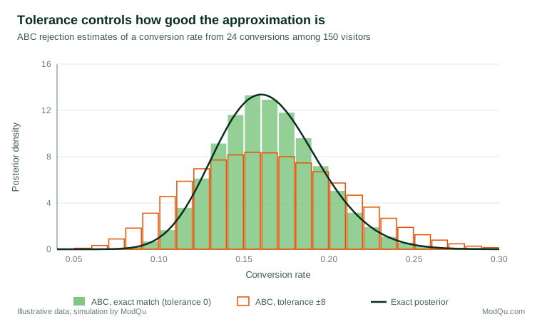
The trade-off is general: smaller tolerances give better approximations but need far more simulations. With complex data, exact matching is impossible, so the data are reduced to summary statistics such as means, variances, correlations or counts. Summaries that discard relevant information produce a posterior that is too wide or even centred in the wrong place. Fearnhead and Prangle (2012) proposed building summaries semi-automatically from regression on pilot simulations, an approach that targets the posterior mean of each parameter.
A further refinement adjusts the accepted values rather than throwing information away. Beaumont et al. (2002) regressed the accepted parameter values on the differences between simulated and observed summaries, then shifted each value to where it would have been if its summaries had matched the data exactly. This local regression adjustment allows a larger tolerance, and therefore fewer wasted simulations, while keeping much of the accuracy of a small one.
A worked example: calibrating a referral model
Consider a hypothetical subscription service that wants to understand how its customers recruit friends. An agent-based simulation represents 5,000 customers on a social network. Each month, a customer recommends the service to each friend with probability r, and a friend who receives a recommendation joins with probability q; there is also a base rate b of joining through advertising. Because recruitment depends on who knows whom and on the timing of earlier sign-ups, the probability of the observed monthly sign-up counts cannot be written down.
The analyst places priors on r, q and b, runs the simulation for 200,000 parameter draws, and summarises each simulated year by three statistics: total sign-ups, the share of sign-ups that came with a referral code, and the month-to-month growth rate in the second half of the year. Draws whose summaries fall within the closest 1% of the observed values are kept. In this illustration the accepted draws show that the base rate b is well determined, while r and q are strongly negatively correlated: the data can tell that the product r × q is about 0.02, but not whether customers recommend often to reluctant friends or rarely to eager ones. That is useful knowledge in itself. It tells the business that a survey asking customers how often they recommend the service would add information the sign-up data cannot supply.
More efficient algorithms
Rejection sampling wastes most simulations when the prior is broad. Marjoram et al. (2003) embedded ABC in Markov chain Monte Carlo, proposing new parameter values near accepted ones. Sequential Monte Carlo versions move a population of parameter values through a series of shrinking tolerances, reusing what was learned at each stage (Sisson et al., 2007; Beaumont et al., 2009). These methods can reduce the number of simulations needed by orders of magnitude. More recent simulation-based inference methods use neural networks to learn the likelihood or posterior from simulations (Cranmer et al., 2020).
Uses in business and research
ABC is suited to models that are built to mimic a process rather than to fit a convenient distribution.
- Agent-based and network models. The parameters of a model of how a product spreads through social ties can be calibrated to observed adoption curves.
- Operations. Arrival and service parameters of a queueing simulation can be inferred from observed waiting times.
- Epidemiology and ecology. Transmission and population models are classic applications (Csilléry et al., 2010).
- Survey processes. A simulation of contact attempts and response behaviour can be calibrated to fieldwork outcomes to explore how design changes might affect response.
Limitations
- Approximation error is hard to judge. Results depend on the tolerance, the distance measure and the summaries. Repeating the analysis with different choices, and checking the method on simulated data where the truth is known, is essential.
- Model choice is fragile. Comparing models with ABC can give misleading answers when the summaries are not sufficient for the comparison (Robert et al., 2011).
- Computation. Each simulation may be slow, and millions may be required.
- The model still matters. ABC fits the model to the data; it cannot show that the model's mechanism is right.
Key takeaways
Approximate Bayesian computation makes Bayesian inference possible for models that can be simulated but not written as a likelihood. Its accuracy depends on the tolerance and summary statistics, which should be chosen deliberately and tested. Used with care, ABC lets complex, realistic models of customers, markets and processes be calibrated to real data, with honest statements of uncertainty.
References
Beaumont, M. A., Cornuet, J.-M., Marin, J.-M., & Robert, C. P. (2009). Adaptive approximate Bayesian computation. Biometrika, 96(4), 983–990. https://doi.org/10.1093/biomet/asp052
Beaumont, M. A., Zhang, W., & Balding, D. J. (2002). Approximate Bayesian computation in population genetics. Genetics, 162(4), 2025–2035. https://doi.org/10.1093/genetics/162.4.2025
Cranmer, K., Brehmer, J., & Louppe, G. (2020). The frontier of simulation-based inference. Proceedings of the National Academy of Sciences, 117(48), 30055–30062. https://doi.org/10.1073/pnas.1912789117
Csilléry, K., Blum, M. G. B., Gaggiotti, O. E., & François, O. (2010). Approximate Bayesian computation (ABC) in practice. Trends in Ecology & Evolution, 25(7), 410–418. https://doi.org/10.1016/j.tree.2010.04.001
Fearnhead, P., & Prangle, D. (2012). Constructing summary statistics for approximate Bayesian computation: Semi-automatic approximate Bayesian computation. Journal of the Royal Statistical Society Series B: Statistical Methodology, 74(3), 419–474. https://doi.org/10.1111/j.1467-9868.2011.01010.x
Marin, J.-M., Pudlo, P., Robert, C. P., & Ryder, R. J. (2012). Approximate Bayesian computational methods. Statistics and Computing, 22(6), 1167–1180. https://doi.org/10.1007/s11222-011-9288-2
Marjoram, P., Molitor, J., Plagnol, V., & Tavaré, S. (2003). Markov chain Monte Carlo without likelihoods. Proceedings of the National Academy of Sciences, 100(26), 15324–15328. https://doi.org/10.1073/pnas.0306899100
Pritchard, J. K., Seielstad, M. T., Perez-Lezaun, A., & Feldman, M. W. (1999). Population growth of human Y chromosomes: A study of Y chromosome microsatellites. Molecular Biology and Evolution, 16(12), 1791–1798. https://doi.org/10.1093/oxfordjournals.molbev.a026091
Robert, C. P., Cornuet, J.-M., Marin, J.-M., & Pillai, N. S. (2011). Lack of confidence in approximate Bayesian computation model choice. Proceedings of the National Academy of Sciences, 108(37), 15112–15117. https://doi.org/10.1073/pnas.1102900108
Rubin, D. B. (1984). Bayesianly justifiable and relevant frequency calculations for the applied statistician. The Annals of Statistics, 12(4), 1151–1172. https://doi.org/10.1214/aos/1176346785
Sisson, S. A., Fan, Y., & Tanaka, M. M. (2007). Sequential Monte Carlo without likelihoods. Proceedings of the National Academy of Sciences, 104(6), 1760–1765. https://doi.org/10.1073/pnas.0607208104
Tavaré, S., Balding, D. J., Griffiths, R. C., & Donnelly, P. (1997). Inferring coalescence times from DNA sequence data. Genetics, 145(2), 505–518. https://doi.org/10.1093/genetics/145.2.505